
Blame
|
1 | # 1. Mathematical refresher |
||||||
| 2 | ||||||||
| 3 | This module gathers the mathematical tools the rest of the course leans on: a little linear algebra, the language of expectation and covariance, the multivariate Gaussian, and the four probability quantities (likelihood, prior, posterior, evidence) that the next module turns into a way of reasoning. It is a reference to return to, not a full treatment. |
|||||||
| 4 | ||||||||
| 5 | ## 1.1 Linear algebra |
|||||||
| 6 | ||||||||
| 7 | A feature vector lives in $\mathbb{R}^n$ and a dataset stacks such vectors into a matrix. The dot product of two vectors sums their elementwise products: |
|||||||
| 8 | ||||||||
| 9 | $$\boxed{ x^T y = \sum_{i=1}^{n} x_i\, y_i }$$ |
|||||||
| 10 | ||||||||
| 11 | A matrix $A$ maps a vector by the matrix-vector product $Ax$, the transpose $A^T$ swaps rows and columns, and the inverse $A^{-1}$ (when it exists) undoes $A$, so $A^{-1}A = I$. The Euclidean norm measures length: |
|||||||
| 12 | ||||||||
| 13 | $$\boxed{ \lVert x \rVert_2 = \sqrt{x^T x} }$$ |
|||||||
| 14 | ||||||||
| 15 | A square matrix is symmetric if $A = A^T$, and positive semidefinite if $x^T A x \ge 0$ for every $x$. Covariance matrices, which appear next, are always symmetric and positive semidefinite. |
|||||||
| 16 | ||||||||
| 17 | ## 1.2 Expectation and variance |
|||||||
| 18 | ||||||||
| 19 | The expectation is the probability-weighted average of a random variable, a sum in the discrete case and an integral in the continuous one: |
|||||||
| 20 | ||||||||
| 21 | $$\boxed{ \mathbb{E}[X] = \sum_x x\, p(x) \qquad \mathbb{E}[X] = \int x\, p(x)\, dx }$$ |
|||||||
| 22 | ||||||||
| 23 | Expectation is linear, $\mathbb{E}[aX + b] = a\,\mathbb{E}[X] + b$. The variance measures spread around the mean $\mu = \mathbb{E}[X]$: |
|||||||
| 24 | ||||||||
| 25 | $$\boxed{ \mathrm{Var}(X) = \mathbb{E}\!\left[(X - \mu)^2\right] = \mathbb{E}[X^2] - \mu^2 }$$ |
|||||||
| 26 | ||||||||
| 27 | ## 1.3 Covariance and the covariance matrix |
|||||||
| 28 | ||||||||
| 29 | Covariance measures how two variables move together: |
|||||||
| 30 | ||||||||
| 31 | $$\boxed{ \mathrm{Cov}(X, Y) = \mathbb{E}\!\left[(X - \mu_X)(Y - \mu_Y)\right] }$$ |
|||||||
| 32 | ||||||||
| 33 | For a random vector $x \in \mathbb{R}^n$ with mean $\mu$, the covariance matrix collects every pairwise covariance: |
|||||||
| 34 | ||||||||
| 35 | $$\boxed{ \Sigma = \mathbb{E}\!\left[(x - \mu)(x - \mu)^T\right], \qquad \Sigma_{ij} = \mathrm{Cov}(x_i, x_j) }$$ |
|||||||
| 36 | ||||||||
| 37 | Its diagonal holds the per-feature variances, it is symmetric, and it is positive semidefinite. Off-diagonal entries record correlation between features. |
|||||||
| 38 | ||||||||
| 39 | ## 1.4 The multivariate Gaussian |
|||||||
| 40 | ||||||||
| 41 | The Gaussian is the default model for continuous noise and for smooth clouds of points. In $n$ dimensions it is parameterized by a mean vector $\mu$ and a covariance matrix $\Sigma$: |
|||||||
| 42 | ||||||||
| 43 | $$\boxed{ p(x) = \frac{1}{(2\pi)^{n/2}\,|\Sigma|^{1/2}} \exp\!\left(-\tfrac{1}{2}(x - \mu)^T \Sigma^{-1}(x - \mu)\right) }$$ |
|||||||
| 44 | ||||||||
| 45 | Its contours of equal density are ellipsoids centred at $\mu$, and the covariance $\Sigma$ sets their spread and orientation. |
|||||||
| 46 | ||||||||
| 47 | 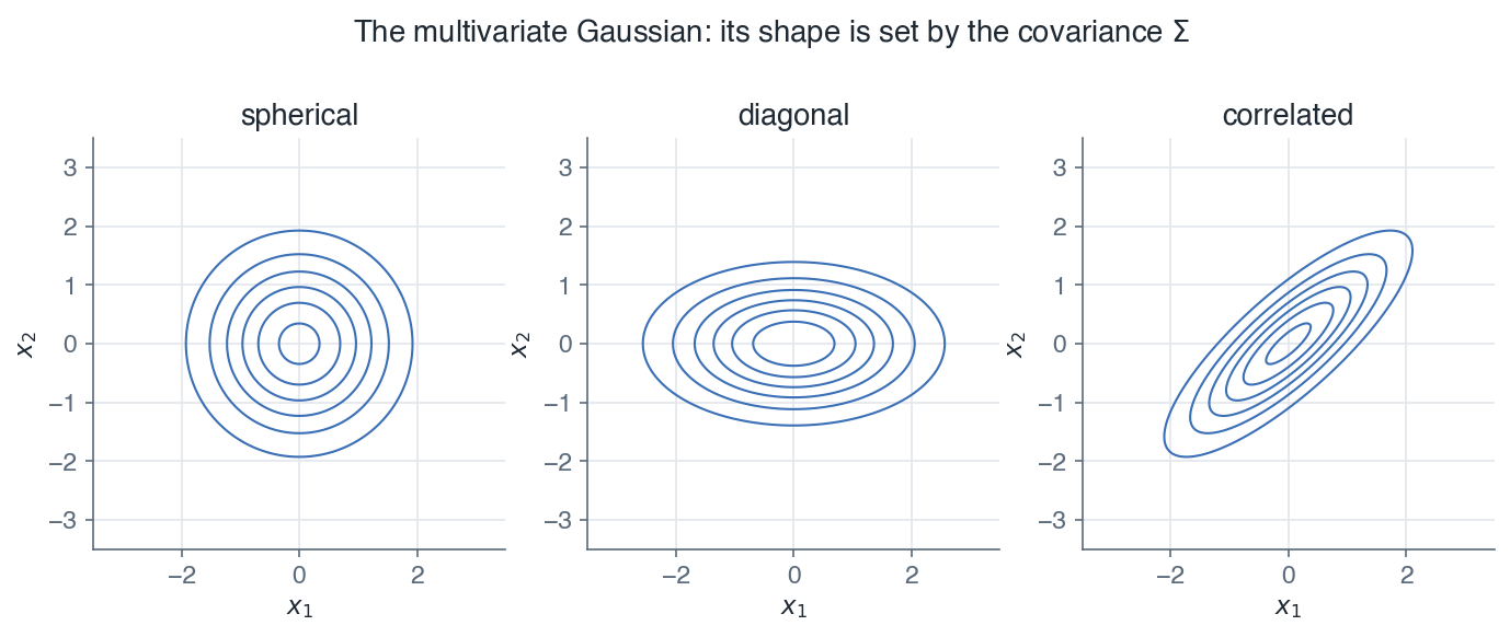 |
|||||||
| 48 | ||||||||
| 49 | *A spherical covariance gives circular contours, a diagonal one gives axis-aligned ellipses, and off-diagonal terms tilt them, encoding correlation between the features.* |
|||||||
| 50 | ||||||||
| 51 | *Remark:* the quadratic form $(x - \mu)^T \Sigma^{-1}(x - \mu)$ is the squared Mahalanobis distance, the natural distance once the data has a covariance structure. |
|||||||
| 52 | ||||||||
| 53 | ## 1.5 Likelihood, prior, posterior, and evidence |
|||||||
| 54 | ||||||||
| 55 | Almost every model in this course reasons about parameters $\theta$ given data $D$. Four quantities recur, and they are tied together by Bayes' rule: |
|||||||
| 56 | ||||||||
| 57 | $$\boxed{ p(\theta \mid D) = \frac{p(D \mid \theta)\, p(\theta)}{p(D)} }$$ |
|||||||
| 58 | ||||||||
| 59 | - The **likelihood** $p(D \mid \theta)$ is how probable the data is under a given $\theta$. |
|||||||
| 60 | - The **prior** $p(\theta)$ is what we believed about $\theta$ before seeing the data. |
|||||||
| 61 | - The **posterior** $p(\theta \mid D)$ is the updated belief after seeing it. |
|||||||
| 62 | - The **evidence** $p(D) = \int p(D \mid \theta)\, p(\theta)\, d\theta$ normalizes the posterior so it integrates to one. |
|||||||
| 63 | ||||||||
| 64 | 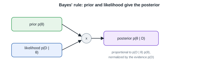 |
|||||||
| 65 | ||||||||
| 66 | *The posterior is proportional to the likelihood times the prior, divided by the evidence that makes it a proper distribution.* |
|||||||
| 67 | ||||||||
| 68 | *Remark:* the evidence is a constant with respect to $\theta$, so for many tasks it can be ignored and only the numerator $p(D \mid \theta)\, p(\theta)$ matters. |
|||||||
| 69 | ||||||||
| 70 | *These tools underpin the [Machine Learning](/en/Machine%20Learning) course, where probability, loss functions, and models are built on them.* |
|||||||
| 71 | ||||||||
| 72 | --- |
|||||||
| 73 | Next: [Course overview](/en/Mathematics) |
|||||||