
1. Mathematical refresher
This module gathers the mathematical tools the rest of the course leans on: a little linear algebra, the language of expectation and covariance, the multivariate Gaussian, and the four probability quantities (likelihood, prior, posterior, evidence) that the next module turns into a way of reasoning. It is a reference to return to, not a full treatment.
1.1 Linear algebra
A feature vector lives in \(\mathbb{R}^n\) and a dataset stacks such vectors into a matrix. The dot product of two vectors sums their elementwise products:
\[\boxed{ x^T y = \sum_{i=1}^{n} x_i\, y_i }\]A matrix \(A\) maps a vector by the matrix-vector product \(Ax\), the transpose \(A^T\) swaps rows and columns, and the inverse \(A^{-1}\) (when it exists) undoes \(A\), so \(A^{-1}A = I\). The Euclidean norm measures length:
\[\boxed{ \lVert x \rVert_2 = \sqrt{x^T x} }\]A square matrix is symmetric if \(A = A^T\), and positive semidefinite if \(x^T A x \ge 0\) for every \(x\). Covariance matrices, which appear next, are always symmetric and positive semidefinite.
1.2 Expectation and variance
The expectation is the probability-weighted average of a random variable, a sum in the discrete case and an integral in the continuous one:
\[\boxed{ \mathbb{E}[X] = \sum_x x\, p(x) \qquad \mathbb{E}[X] = \int x\, p(x)\, dx }\]Expectation is linear, \(\mathbb{E}[aX + b] = a\,\mathbb{E}[X] + b\). The variance measures spread around the mean \(\mu = \mathbb{E}[X]\):
\[\boxed{ \mathrm{Var}(X) = \mathbb{E}\!\left[(X - \mu)^2\right] = \mathbb{E}[X^2] - \mu^2 }\]1.3 Covariance and the covariance matrix
Covariance measures how two variables move together:
\[\boxed{ \mathrm{Cov}(X, Y) = \mathbb{E}\!\left[(X - \mu_X)(Y - \mu_Y)\right] }\]For a random vector \(x \in \mathbb{R}^n\) with mean \(\mu\), the covariance matrix collects every pairwise covariance:
\[\boxed{ \Sigma = \mathbb{E}\!\left[(x - \mu)(x - \mu)^T\right], \qquad \Sigma_{ij} = \mathrm{Cov}(x_i, x_j) }\]Its diagonal holds the per-feature variances, it is symmetric, and it is positive semidefinite. Off-diagonal entries record correlation between features.
1.4 The multivariate Gaussian
The Gaussian is the default model for continuous noise and for smooth clouds of points. In \(n\) dimensions it is parameterized by a mean vector \(\mu\) and a covariance matrix \(\Sigma\):
\[\boxed{ p(x) = \frac{1}{(2\pi)^{n/2}\,|\Sigma|^{1/2}} \exp\!\left(-\tfrac{1}{2}(x - \mu)^T \Sigma^{-1}(x - \mu)\right) }\]
Its contours of equal density are ellipsoids centred at \(\mu\), and the covariance \(\Sigma\) sets their spread and orientation.
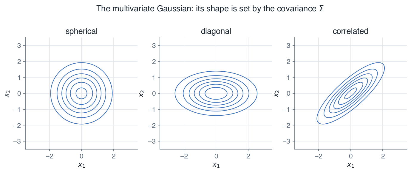
A spherical covariance gives circular contours, a diagonal one gives axis-aligned ellipses, and off-diagonal terms tilt them, encoding correlation between the features.
Remark: the quadratic form \((x - \mu)^T \Sigma^{-1}(x - \mu)\) is the squared Mahalanobis distance, the natural distance once the data has a covariance structure.
1.5 Likelihood, prior, posterior, and evidence
Almost every model in this course reasons about parameters \(\theta\) given data \(D\). Four quantities recur, and they are tied together by Bayes' rule:
\[\boxed{ p(\theta \mid D) = \frac{p(D \mid \theta)\, p(\theta)}{p(D)} }\]- The likelihood \(p(D \mid \theta)\) is how probable the data is under a given \(\theta\).
- The prior \(p(\theta)\) is what we believed about \(\theta\) before seeing the data.
- The posterior \(p(\theta \mid D)\) is the updated belief after seeing it.
- The evidence \(p(D) = \int p(D \mid \theta)\, p(\theta)\, d\theta\) normalizes the posterior so it integrates to one.
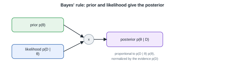
The posterior is proportional to the likelihood times the prior, divided by the evidence that makes it a proper distribution.
Remark: the evidence is a constant with respect to \(\theta\), so for many tasks it can be ignored and only the numerator \(p(D \mid \theta)\, p(\theta)\) matters.
These tools underpin the Machine Learning course, where probability, loss functions, and models are built on them.
Next: Course overview