Commit e0287e

2026-07-02 15:52:15 lugonthier: Add new content and images for machine learning and mathematics modules - Added images for regularization and high-dimensional inference. - Introduced Support Vector Machines (SVM) module with detailed explanations and images. - Created Decision Trees and Ensemble Methods module with comprehensive content and illustrations. - Added a Mathematics overview module and a refresher on mathematical concepts essential for machine learning. - Included SVG diagrams for Bayes' rule and multivariate Gaussian distribution.

en.md ..
@@ 1,10 1,11 @@
	# ML & MLOps Courses
-	Three courses on machine learning, deep learning, and putting models into production. Use the flags
-	in the top bar to change language.
+	Four courses covering the mathematics behind machine learning, the core ML and deep learning methods,
+	and putting models into production. Use the flags in the top bar to change language.
	## Courses
+	- [Mathematics](/en/Mathematics): the linear algebra and probability the courses build on.
	- [Machine Learning](/en/Machine%20Learning): foundations of ML, from data to models.
	- [Deep Learning](/en/Deep%20Learning): neural networks from the perceptron to transformers.
	- [MLOps](/en/MLOps): taking ML systems to production and keeping them healthy.
en/Deep Learning.md ..
@@ 2,7 2,7 @@
	Neural networks from the single perceptron to modern transformers: how depth, the right activations, and gradient-based training let a model learn its own features instead of hand-crafted ones.
-	**Prerequisites:** the [Machine Learning](/en/Machine%20Learning) course (especially the perceptron in [Linear models](/en/Machine%20Learning/04%20Linear%20models)), basic Python, calculus, and linear algebra.
+	**Prerequisites:** the [Machine Learning](/en/Machine%20Learning) course (especially the perceptron in [Linear classification](/en/Machine%20Learning/06%20Linear%20classification)), basic Python, calculus, and linear algebra.
	## Syllabus
en/Deep Learning/01 Introduction.md ..
@@ 1,6 1,6 @@
	# 1. Introduction
-	This course continues directly from the Machine Learning course, which closed the [Linear models](/en/Machine%20Learning/04%20Linear%20models) part with a key remark: a perceptron is a single unit, and stacked into layers it becomes a neural network. This lesson makes that bridge explicit. It recalls what one unit can do, shows the concrete task (XOR) where a single unit fails, and fixes the notation used throughout the rest of the course.
+	This course continues directly from the Machine Learning course, which closed the [Linear classification](/en/Machine%20Learning/06%20Linear%20classification) part with a key remark: a perceptron is a single unit, and stacked into layers it becomes a neural network. This lesson makes that bridge explicit. It recalls what one unit can do, shows the concrete task (XOR) where a single unit fails, and fixes the notation used throughout the rest of the course.
	**Objectives**
	- Recall the perceptron as a single unit with a step activation and a linear boundary.
en/Machine Learning.md ..
@@ 2,17 2,19 @@
	Foundations of machine learning: how to go from raw data to a trained, evaluated model.
-	**Prerequisites:** basic Python, basic linear algebra and statistics.
+	**Prerequisites:** basic Python and the [Mathematics](/en/Mathematics) course (linear algebra, probability, statistics).
	## Syllabus
	1. [Introduction](/en/Machine%20Learning/01%20Introduction)
	2. [General concepts](/en/Machine%20Learning/02%20General%20concepts)
	3. [Model evaluation and validation](/en/Machine%20Learning/03%20Model%20evaluation%20and%20validation)
-	4. [Linear models](/en/Machine%20Learning/04%20Linear%20models)
-	5. [Regularization and high-dimensional inference](/en/Machine%20Learning/05%20Regularization%20and%20high-dimensional%20inference)
-	6. [Support Vector Machines](/en/Machine%20Learning/06%20Support%20Vector%20Machines)
-	7. [Decision trees and ensemble methods](/en/Machine%20Learning/07%20Decision%20trees%20and%20ensemble%20methods)
+	4. [Probabilistic formulation](/en/Machine%20Learning/04%20Probabilistic%20formulation)
+	5. [Linear regression](/en/Machine%20Learning/05%20Linear%20regression)
+	6. [Linear classification](/en/Machine%20Learning/06%20Linear%20classification)
+	7. [Regularization and high-dimensional inference](/en/Machine%20Learning/07%20Regularization%20and%20high-dimensional%20inference)
+	8. [Support Vector Machines](/en/Machine%20Learning/08%20Support%20Vector%20Machines)
+	9. [Decision trees and ensemble methods](/en/Machine%20Learning/09%20Decision%20trees%20and%20ensemble%20methods)
	---
	[MLOps](/en/MLOps) · [Home](/en)
en/Machine Learning/03 Model evaluation and validation.md ..
@@ 70,4 70,4 @@
	*With a way to measure generalization in hand, the next module fits our first models, and the one after controls their complexity with regularization tuned by exactly this cross-validation.*
	---
-	Next: [Linear models](/en/Machine%20Learning/04%20Linear%20models) · [Course overview](/en/Machine%20Learning)
+	Next: [Probabilistic formulation](/en/Machine%20Learning/04%20Probabilistic%20formulation) · [Course overview](/en/Machine%20Learning)
en/Machine Learning/04 Linear models.md .. /dev/null
@@ 1,193 0,0 @@
-	# 4. Linear models
-
-	Linear models predict from a linear score $\theta^T x$. This module covers linear regression (continuous targets), logistic regression (binary classification), and the generalized linear model framework that unifies both through the exponential family. Each model is fit by maximum likelihood and shares the same gradient-based update.
-
-	**Objectives**
-	- Define the linear hypothesis and fit $\theta$ by the LMS update or the closed-form normal equation.
-	- See why least squares is the maximum-likelihood estimate under Gaussian noise.
-	- Map the linear score through the sigmoid and fit it by gradient ascent or Newton's method.
-	- Classify with the perceptron and know when its learning rule converges.
-	- Recognize the exponential-family form and build a GLM from its three assumptions.
-	- Recover linear, logistic, and softmax regression as special cases.
-
-	## 4.1 Linear regression
-
-	### 4.1.1 Hypothesis
-
-	The hypothesis is linear in the augmented input $x \in \mathbb{R}^{n+1}$ with $x_0 = 1$ and parameters $\theta \in \mathbb{R}^{n+1}$:
-
-	$$\boxed{ h_\theta(x) = \theta^T x }$$
-
-	### 4.1.2 Cost function
-
-	The cost is defined as half the sum of squared residuals over the $m$ examples:
-
-	$$\boxed{ J(\theta) = \tfrac{1}{2}\sum_{i=1}^{m}\left(h_\theta(x^{(i)}) - y^{(i)}\right)^2 }$$
-
-	### 4.1.3 LMS update
-
-	Gradient descent on $J$ gives the least-mean-squares (Widrow-Hoff) update, applied per example $(x^{(i)}, y^{(i)})$:
-
-	$$\boxed{ \theta_j \leftarrow \theta_j + \alpha\left(y^{(i)} - h_\theta(x^{(i)})\right)x_j^{(i)} }$$
-
-	with learning rate $\alpha > 0$.
-
-	| variant | update rule | per step | use when |
-	| --- | --- | --- | --- |
-	| Batch GD | sum over all $m$ examples | $O(mn)$ | $m$ small to moderate |
-	| Stochastic GD (SGD) | one example at a time | $O(n)$ | $m$ large, streaming |
-
-	### 4.1.4 Normal equation
-
-	Setting $\nabla_\theta J(\theta) = 0$ gives a closed-form solution from the design matrix $X$ and target vector $y$:
-
-	$$\boxed{ \theta = (X^T X)^{-1}X^T y }$$
-
-	*Remark:* the normal equation needs no learning rate and no iteration, but inverting $X^T X$ costs $O(n^3)$, so for large $n$ the iterative LMS update is preferred.
-
-	### 4.1.5 Probabilistic interpretation
-
-	Assume $y^{(i)} = \theta^T x^{(i)} + \varepsilon^{(i)}$ with i.i.d. Gaussian noise $\varepsilon^{(i)} \sim \mathcal{N}(0, \sigma^2)$. Maximizing the log-likelihood then coincides with minimizing the least-squares cost:
-
-	$$\boxed{ \arg\max_\theta \ell(\theta) = \arg\min_\theta J(\theta) }$$
-
-	*Remark:* this is why least squares is a principled objective and not merely a convenient one.
-
-	
-
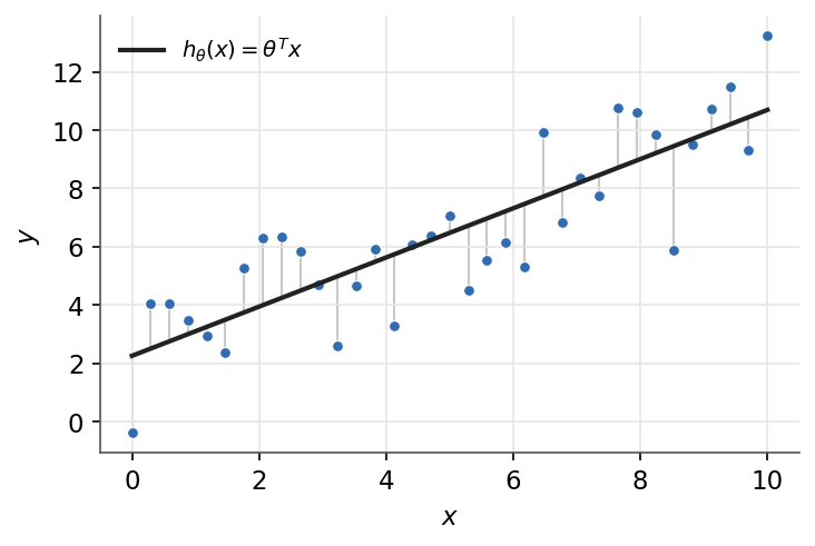
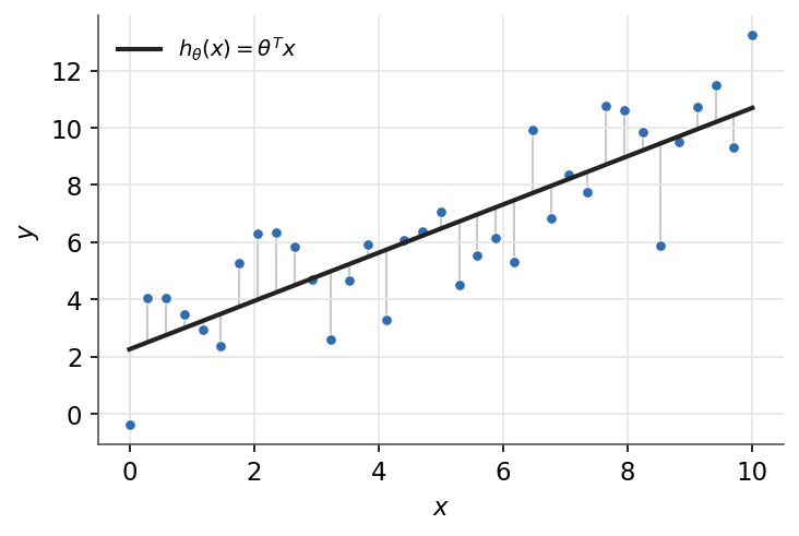
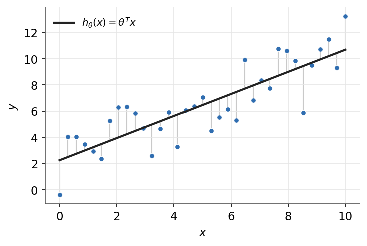
-	*Least squares fits the line that minimizes the squared residuals (grey segments).*
-
-	## 4.2 Logistic regression
-
-	### 4.2.1 Sigmoid
-
-	The sigmoid (logistic) function squashes a raw score $z \in \mathbb{R}$ into a probability:
-
-	$$\boxed{ g(z) = \frac{1}{1 + e^{-z}} \in (0, 1) }$$
-
-	Its derivative has the convenient form $g'(z) = g(z)\left(1 - g(z)\right)$.
-
-	### 4.2.2 Model
-
-	The hypothesis outputs the probability of the positive class, with $\phi$ the predicted probability:
-
-	$$\boxed{ \phi = h_\theta(x) = g(\theta^T x) = p(y = 1 \mid x; \theta) }$$
-
-	Labels are $y \in \{0, 1\}$, so the conditional law is Bernoulli:
-
-	$$\boxed{ p(y \mid x; \theta) = \phi^{y}(1 - \phi)^{1 - y} }$$
-
-	### 4.2.3 Log-likelihood
-
-	Over $m$ i.i.d. examples the log-likelihood is the negative cross-entropy summed over the data:
-
-	$$\boxed{ \ell(\theta) = \sum_{i=1}^{m}\left[ y^{(i)}\log \phi^{(i)} + (1 - y^{(i)})\log(1 - \phi^{(i)}) \right] }$$
-
-	with $\phi^{(i)} = h_\theta(x^{(i)})$.
-
-	### 4.2.4 Gradient ascent
-
-	Maximizing $\ell$ by gradient ascent gives the same form as the LMS update:
-
-	$$\boxed{ \theta_j \leftarrow \theta_j + \alpha\left(y^{(i)} - h_\theta(x^{(i)})\right)x_j^{(i)} }$$
-
-	*Remark:* the update matches linear regression in form, even though $h_\theta$ is now the sigmoid. This is no coincidence, both are generalized linear models.
-
-	### 4.2.5 Newton's method
-
-	Newton's method converges faster near the optimum. In one dimension:
-
-	$$\boxed{ \theta \leftarrow \theta - \frac{\ell'(\theta)}{\ell''(\theta)} }$$
-
-	In the vector case it uses the Hessian $H$ of $\ell$:
-
-	$$\boxed{ \theta \leftarrow \theta - H^{-1}\nabla_\theta \ell(\theta) }$$
-
-	*Remark:* logistic regression has no closed-form solution for $\theta$, so it is always fit iteratively (gradient ascent or Newton).
-
-	
-
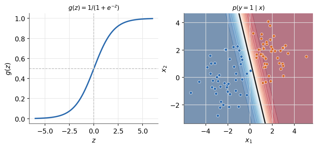
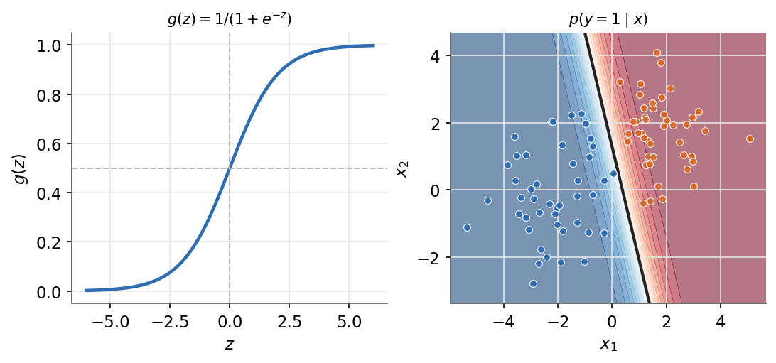
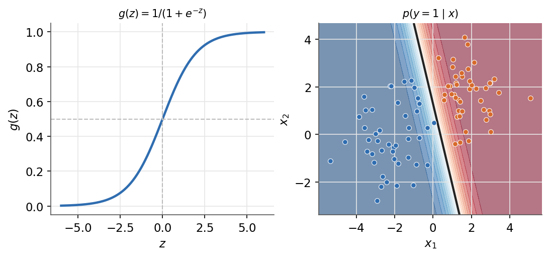
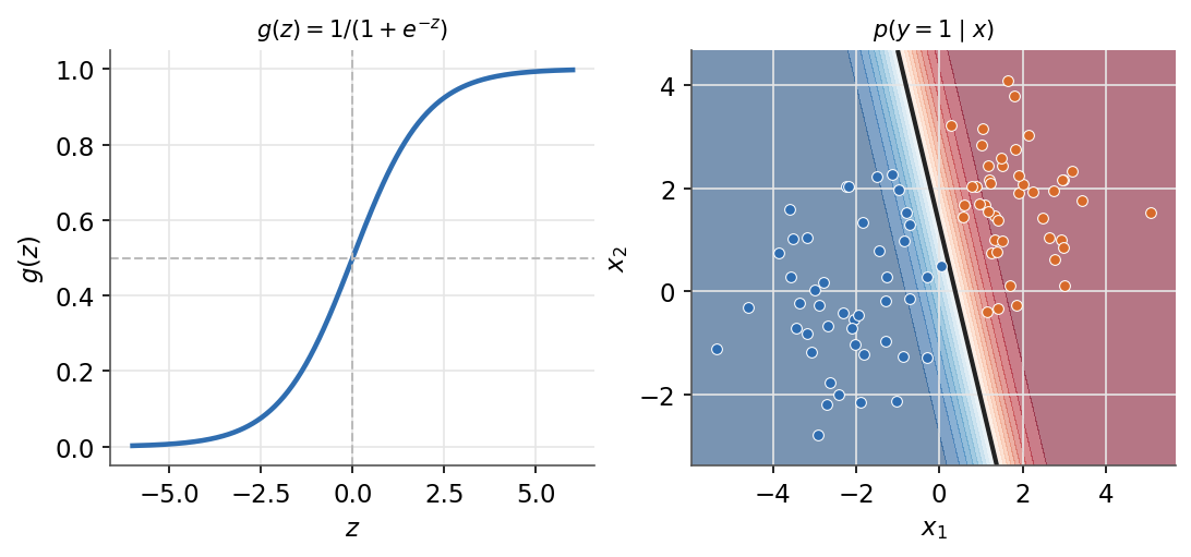
-	*Left: the sigmoid maps scores into the interval (0,1). Right: the decision boundary and predicted probability.*
-
-	## 4.3 Perceptron
-
-	The perceptron is the original linear classifier. It keeps the linear score $\theta^T x$ of logistic regression but replaces the sigmoid with a hard threshold, so the output is a class label rather than a probability. Labels are $y \in \{0, 1\}$.
-
-	### 4.3.1 Activation and hypothesis
-
-	The activation is the step function:
-
-	$$\boxed{ g(z) = \begin{cases} 1 & \text{if } z \ge 0 \\ 0 & \text{otherwise} \end{cases} }$$
-
-	and the hypothesis applies it to the linear score:
-
-	$$\boxed{ h_\theta(x) = g(\theta^T x) }$$
-
-	### 4.3.2 Learning rule
-
-	The perceptron is trained online, one example at a time, and corrects $\theta$ only on a misclassified point:
-
-	$$\boxed{ \theta_j \leftarrow \theta_j + \alpha\left(y^{(i)} - h_\theta(x^{(i)})\right)x_j^{(i)} }$$
-
-	*Remark:* this is the same form as the LMS update and the logistic gradient-ascent update. Only the activation $g$ differs (identity, sigmoid, step). When the prediction is right the factor $y^{(i)} - h_\theta(x^{(i)})$ is zero, so correctly classified points leave $\theta$ unchanged.
-
-	
-
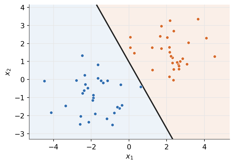
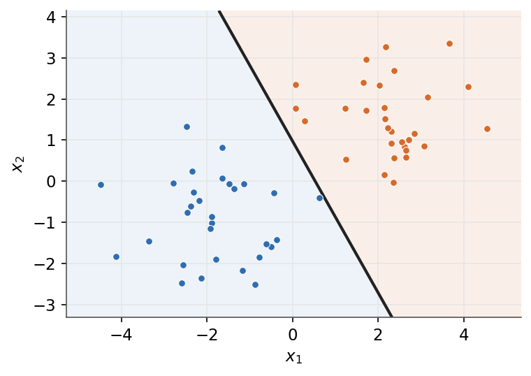
-	*The perceptron finds one separating hyperplane. It is not necessarily the maximum-margin one the SVM will choose.*
-
-	### 4.3.3 Convergence
-
-	| data | behaviour |
-	| --- | --- |
-	| linearly separable | converges in a finite number of updates |
-	| not separable | never converges, the weights keep oscillating |
-
-	*Remark:* the perceptron stops at the first hyperplane that separates the data, usually not the one with the widest margin. This gap motivates the support vector machine (which maximizes the margin) and, stacked into layers, the neural network (a perceptron is a single unit).
-
-	## 4.4 Generalized linear models
-
-	### 4.4.1 Exponential family
-
-	A distribution is in the exponential family if its density can be written with natural parameter $\eta$, sufficient statistic $T(y)$, log-partition $a(\eta)$, and base measure $b(y)$:
-
-	$$\boxed{ p(y; \eta) = b(y)\exp\left(\eta\, T(y) - a(\eta)\right) }$$
-
-	### 4.4.2 GLM assumptions
-
-	A GLM rests on three choices. The response is in the exponential family, the natural parameter is linear in the input, and the prediction is the expected sufficient statistic:
-
-	$$\boxed{ \eta = \theta^T x }$$
-
-	$$\boxed{ h_\theta(x) = \mathbb{E}\left[T(y) \mid x; \theta\right] }$$
-
-	### 4.4.3 Family table
-
-	| Distribution | $\eta$ | $T(y)$ | $a(\eta)$ | $b(y)$ |
-	| --- | --- | --- | --- | --- |
-	| Bernoulli | $\log\dfrac{\phi}{1-\phi}$ | $y$ | $\log(1 + e^{\eta})$ | $1$ |
-	| Gaussian ($\sigma^2 = 1$) | $\mu$ | $y$ | $\tfrac{1}{2}\eta^2$ | $\dfrac{1}{\sqrt{2\pi}}e^{-y^2/2}$ |
-	| Poisson | $\log\lambda$ | $y$ | $e^{\eta}$ | $\dfrac{1}{y!}$ |
-	| Geometric | $\log(1-\phi)$ | $y$ | $\log\dfrac{e^{\eta}}{1 - e^{\eta}}$ | $1$ |
-
-	*Remark:* for the Bernoulli, $\eta$ is the log-odds and its inverse is the sigmoid, $\phi = g(\eta)$. This is why logistic regression has the form it does.
-
-	### 4.4.4 Softmax regression
-
-	For multiclass labels $y \in \{1, \dots, k\}$ the GLM gives softmax regression, with one parameter vector $\theta_k$ per class:
-
-	$$\boxed{ p(y = k \mid x; \theta) = \frac{\exp(\theta_k^T x)}{\sum_{j}\exp(\theta_j^T x)} }$$
-
-	### 4.4.5 GLM recipe
-
-	```mermaid
-	graph TD
-	A["pick a response distribution"] --> B["write it in exponential-family form"]
-	B --> C["set natural parameter eta linear in x"]
-	C --> D["prediction is expected sufficient statistic"]
-	D --> E["fit theta by maximum likelihood"]
-	```
-
-	*Linear models, including the perceptron, settle for any boundary that separates the classes. The next part asks for the best one: the support vector machine maximizes the margin.*
-
-	---
-	Next: [Regularization and high-dimensional inference](/en/Machine%20Learning/05%20Regularization%20and%20high-dimensional%20inference) · [Course overview](/en/Machine%20Learning)
/dev/null .. en/Machine Learning/04 Probabilistic formulation.md
@@ 0,0 1,75 @@
+	# 4. Probabilistic formulation
+
+	Probability is the language machine learning uses to handle uncertainty. This module sets out the rules for discrete and continuous variables, takes a first look at information theory, shows the Bayesian way of turning probabilities into decisions, and defines the two estimation principles the course returns to again and again: maximum likelihood and maximum a posteriori.
+
+	**Objectives**
+	- State the rules of probability for discrete and continuous variables.
+	- Relate joint, conditional, and marginal probabilities by the sum and product rules and by Bayes' rule.
+	- Measure uncertainty with entropy, cross-entropy, and the Kullback-Leibler divergence.
+	- Make the decision that minimizes expected loss, and recover the maximum-a-posteriori classifier.
+	- Define the maximum-likelihood and maximum-a-posteriori estimators.
+
+	## 4.1 Probability, discrete and continuous
+
+	A random variable takes values with probabilities that are non-negative and sum or integrate to one. A discrete variable has a probability mass function, a continuous one a probability density function:
+
+	$$\boxed{ \sum_x p(x) = 1 \qquad \int p(x)\, dx = 1, \quad p(x) \ge 0 }$$
+
+	For a continuous variable, probability attaches to intervals through an integral, $P(a \le X \le b) = \int_a^b p(x)\, dx$, not to single points.
+
+	## 4.2 Joint, conditional, and Bayes
+
+	Two variables have a joint distribution $p(x, y)$. Summing (or integrating) out one variable gives the marginal, the sum rule, and the joint factors into a conditional times a marginal, the product rule:
+
+	$$\boxed{ p(x) = \sum_y p(x, y) \qquad p(x, y) = p(y \mid x)\, p(x) }$$
+
+	Rearranging the product rule both ways gives Bayes' rule, which flips a conditional:
+
+	$$\boxed{ p(y \mid x) = \frac{p(x \mid y)\, p(y)}{p(x)} }$$
+
+	Two variables are independent when the joint is the product of the marginals, $p(x, y) = p(x)\, p(y)$.
+
+	## 4.3 A little information theory
+
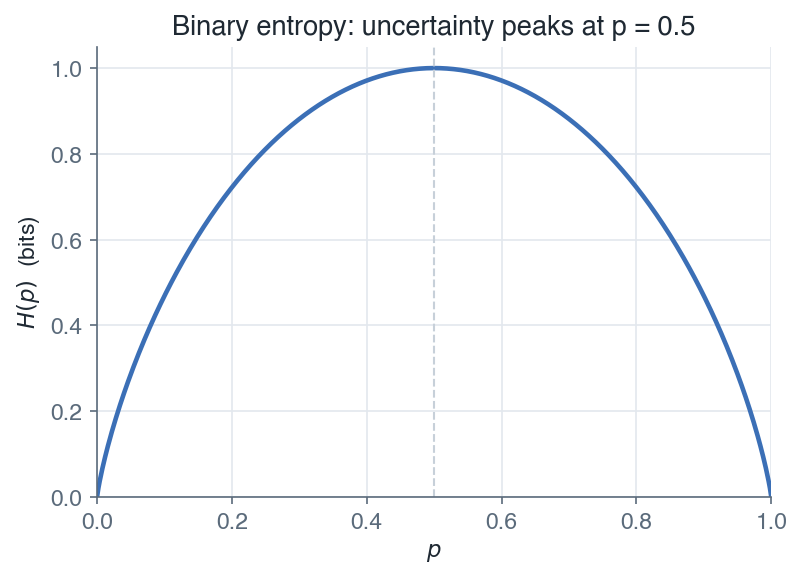
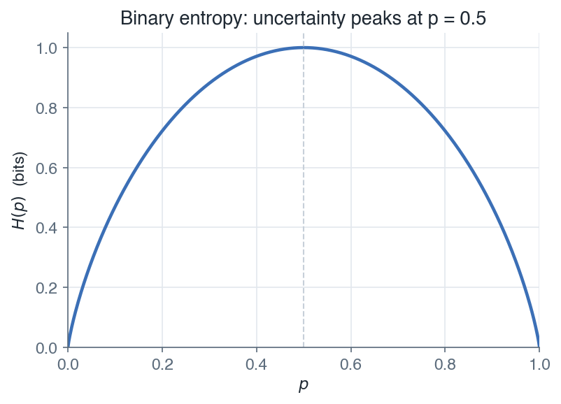
+	The entropy of a distribution measures its uncertainty, the average number of bits needed to describe an outcome:
+
+	$$\boxed{ H(X) = -\sum_x p(x)\log p(x) }$$
+
+	
+
+	*For a two-outcome variable the entropy is largest at $p = 0.5$, where the outcome is hardest to predict, and zero when one outcome is certain.*
+
+	The cross-entropy measures the cost of using a model $q$ when the truth is $p$, and the Kullback-Leibler divergence measures how far $q$ sits from $p$:
+
+	$$\boxed{ H(p, q) = -\sum_x p(x)\log q(x) \qquad D_{\mathrm{KL}}(p \,\|\, q) = \sum_x p(x)\log\frac{p(x)}{q(x)} \ge 0 }$$
+
+	*Remark:* minimizing the cross-entropy between the true labels and a model's predictions is the same as maximizing the likelihood of those labels. This is why classification networks minimize cross-entropy, a thread picked up in later modules.
+
+	## 4.4 Bayesian decision theory
+
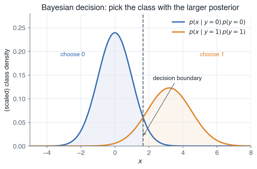
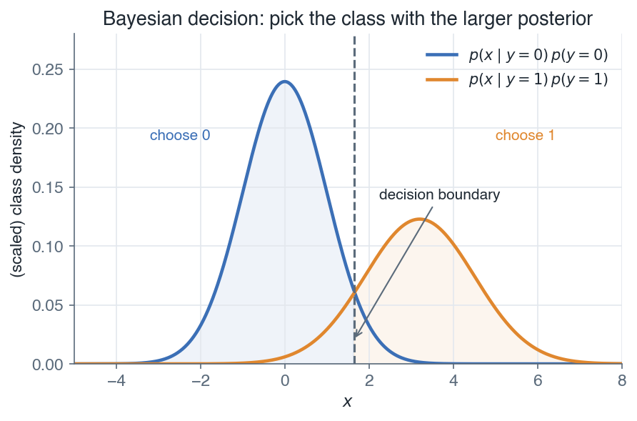
+	To classify an input $x$, the Bayesian rule uses the posterior over classes. Under the 0-1 loss, the decision that minimizes the expected loss is simply the most probable class, and because the posterior is proportional to the class-conditional density times the prior, it can be computed either way:
+
+	$$\boxed{ \hat{y} = \arg\max_y \; p(y \mid x) = \arg\max_y \; p(x \mid y)\, p(y) }$$
+
+	
+
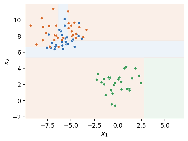
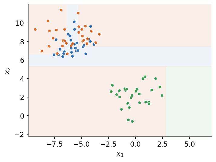
+	*Each class contributes its density scaled by its prior, and the decision boundary falls where the two are equal. On each side the class with the larger posterior wins.*
+
+	*Remark:* this is the optimal classifier, called the Bayes classifier. Every method later in the course is, in effect, an attempt to approximate these posteriors from data.
+
+	## 4.5 Maximum likelihood and maximum a posteriori
+
+	We rarely know the true distribution, so we estimate its parameters $\theta$ from data. Maximum likelihood picks the $\theta$ that makes the observed data most probable, usually maximized as a sum of log-likelihoods over the $m$ examples:
+
+	$$\boxed{ \theta_{\mathrm{MLE}} = \arg\max_\theta \sum_{i=1}^{m} \log p(x^{(i)} \mid \theta) }$$
+
+	Maximum a posteriori instead maximizes the posterior, which multiplies the likelihood by a prior on $\theta$:
+
+	$$\boxed{ \theta_{\mathrm{MAP}} = \arg\max_\theta \; p(D \mid \theta)\, p(\theta) }$$
+
+	*Remark:* maximum a posteriori is maximum likelihood plus a prior. A Gaussian prior on $\theta$ becomes an L2 penalty and a Laplace prior an L1 penalty, which is exactly the regularization of a later module. With abundant data the prior washes out and the two estimators agree.
+
+	*The next module turns these principles into concrete loss functions and the gradient descent that minimizes them.*
+
+	---
+	Next: [Linear regression](/en/Machine%20Learning/05%20Linear%20regression) · [Course overview](/en/Machine%20Learning)
/dev/null .. en/Machine Learning/04 Probabilistic formulation/bayes-decision.png
/dev/null .. en/Machine Learning/04 Probabilistic formulation/entropy.png
/dev/null .. en/Machine Learning/05 Linear regression.md
@@ 0,0 1,62 @@
+	# 5. Linear regression
+
+	Linear regression predicts a continuous target from a linear score $\theta^T x$. This module presents it probabilistically, building on the [Probabilistic formulation](/en/Machine%20Learning/04%20Probabilistic%20formulation) module: the model (extended to polynomial features), fitting by maximum likelihood, which turns out to be ordinary least squares, and fitting by maximum a posteriori, which adds a prior and yields a regularized fit.
+
+	**Objectives**
+	- Write the linear and polynomial regression model and fit it by least squares.
+	- Give regression a probabilistic formulation with Gaussian noise.
+	- See that maximum likelihood under that model is exactly least squares.
+	- Add a prior and fit by maximum a posteriori, recovering a regularized fit.
+
+	## 5.1 The linear and polynomial model
+
+	The hypothesis is linear in the augmented input $x \in \mathbb{R}^{n+1}$ with $x_0 = 1$ and parameters $\theta$:
+
+	$$\boxed{ h_\theta(x) = \theta^T x }$$
+
+	Polynomial regression is the same model applied to a feature map. Replacing $x$ by $\phi(x) = (1, x, x^2, \dots, x^d)$ fits a degree-$d$ polynomial while staying linear in the parameters:
+
+	$$\boxed{ h_\theta(x) = \theta^T \phi(x) = \sum_{j=0}^{d} \theta_j\, x^{j} }$$
+
+	so everything below applies unchanged once the design matrix $X$ stacks the transformed inputs $\phi(x^{(i)})$ as its rows.
+
+	## 5.2 Least squares
+
+	The cost is half the sum of squared residuals over the $m$ examples:
+
+	$$\boxed{ J(\theta) = \tfrac{1}{2}\sum_{i=1}^{m}\left(h_\theta(x^{(i)}) - y^{(i)}\right)^2 }$$
+
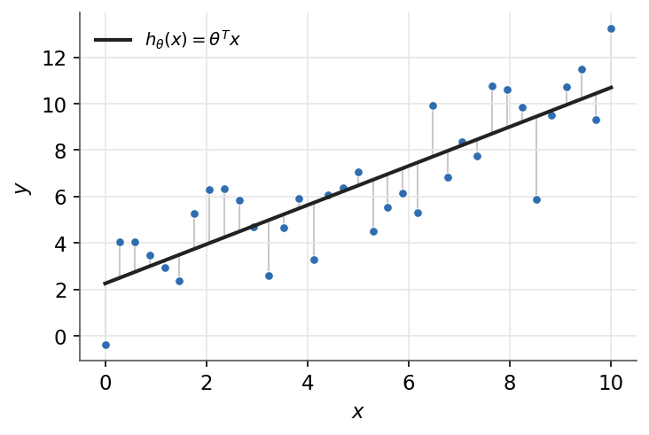
+	Setting $\nabla_\theta J = 0$ gives the closed-form normal equation, and gradient descent gives the equivalent iterative update:
+
+	$$\boxed{ \theta = (X^T X)^{-1}X^T y \qquad \theta_j \leftarrow \theta_j + \alpha\left(y^{(i)} - h_\theta(x^{(i)})\right)x_j^{(i)} }$$
+
+	
+
+	*Least squares fits the curve that minimizes the squared residuals (grey segments).*
+
+	## 5.3 Probabilistic formulation: maximum likelihood
+
+	Give the data a generative story: each target is the linear prediction plus independent Gaussian noise,
+
+	$$\boxed{ y^{(i)} = \theta^T x^{(i)} + \varepsilon^{(i)}, \quad \varepsilon^{(i)} \sim \mathcal{N}(0, \sigma^2) }$$
+
+	so $p(y^{(i)} \mid x^{(i)}; \theta) = \mathcal{N}(\theta^T x^{(i)}, \sigma^2)$. Maximizing the log-likelihood over the $m$ i.i.d. examples drops every term that does not depend on $\theta$ and leaves the least-squares cost:
+
+	$$\boxed{ \arg\max_\theta \ell(\theta) = \arg\min_\theta \sum_{i=1}^{m}\left(y^{(i)} - \theta^T x^{(i)}\right)^2 }$$
+
+	*Remark:* this is why least squares is a principled objective and not merely a convenient one. Ordinary least squares is the maximum-likelihood estimate under Gaussian noise, exactly the maximum-likelihood principle from the previous module.
+
+	## 5.4 Maximum a posteriori
+
+	Maximum likelihood can overfit, especially at high polynomial degree. Placing a zero-mean Gaussian prior on the parameters, $\theta \sim \mathcal{N}(0, \tau^2 I)$, and maximizing the posterior instead adds a penalty on their size:
+
+	$$\boxed{ \theta_{\mathrm{MAP}} = \arg\min_\theta \; \sum_{i=1}^{m}\left(y^{(i)} - \theta^T x^{(i)}\right)^2 + \lambda \lVert \theta \rVert_2^2, \quad \lambda = \frac{\sigma^2}{\tau^2} }$$
+
+	This is regularized (ridge) regression: the Gaussian prior becomes an L2 penalty, exactly the prior-to-penalty link noted in the previous module.
+
+	*Remark:* a stronger prior (small $\tau$) means a larger $\lambda$ and more shrinkage toward zero. With abundant data the likelihood dominates the prior and the maximum-a-posteriori fit approaches the maximum-likelihood one. Choosing the degree $d$ and the penalty $\lambda$ is a model-selection problem, settled by cross-validation from the [evaluation module](/en/Machine%20Learning/03%20Model%20evaluation%20and%20validation), and taken further in the [regularization module](/en/Machine%20Learning/07%20Regularization%20and%20high-dimensional%20inference).
+
+	*The same linear score, passed through a squashing function instead of read directly, turns regression into classification, the subject of the next module.*
+
+	---
+	Next: [Linear classification](/en/Machine%20Learning/06%20Linear%20classification) · [Course overview](/en/Machine%20Learning)
en/Machine Learning/04 Linear models/linear-regression.png .. en/Machine Learning/05 Linear regression/linear-regression.png
/dev/null .. en/Machine Learning/06 Linear classification.md
@@ 0,0 1,83 @@
+	# 6. Linear classification
+
+	Classification predicts a discrete label from the same linear score $\theta^T x$. This module starts from the idea of treating classification as regression, then builds the two classical linear classifiers: the perceptron, binary and multiclass, and logistic regression, binary with the sigmoid and multiclass with the softmax, all trained by gradient descent on the cross-entropy loss.
+
+	**Objectives**
+	- See why regressing the labels directly is a poor classifier, and how a squashing function fixes it.
+	- Classify with the perceptron, binary and multiclass, and know when it converges.
+	- Fit binary logistic regression with the sigmoid and the cross-entropy loss.
+	- Extend to many classes with the softmax, and relate the sigmoid and the softmax.
+	- Train these models by gradient descent.
+
+	## 6.1 Classification as a regression problem
+
+	One could fit least squares to the labels $y \in \{0, 1\}$ directly, but the linear output is unbounded, is pulled around by outliers, and does not read as a probability. The fix is to keep the linear score and pass it through a squashing function that maps it to a class or a probability. The rest of the module is two choices of that function.
+
+	## 6.2 The perceptron
+
+	### 6.2.1 Binary perceptron
+
+	The perceptron passes the score through a hard step, so the output is a class label:
+
+	$$\boxed{ h_\theta(x) = g(\theta^T x), \quad g(z) = \begin{cases} 1 & \text{if } z \ge 0 \\ 0 & \text{otherwise} \end{cases} }$$
+
+	It is trained online, correcting $\theta$ only on a misclassified point:
+
+	$$\boxed{ \theta_j \leftarrow \theta_j + \alpha\left(y^{(i)} - h_\theta(x^{(i)})\right)x_j^{(i)} }$$
+
+	
+
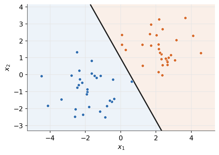
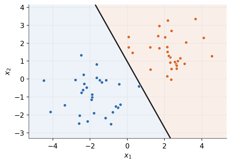
+	*The perceptron finds one separating hyperplane, not necessarily the maximum-margin one the support vector machine will choose.*
+
+	### 6.2.2 Multiclass perceptron
+
+	With $k$ classes, keep one weight vector $\theta_c$ per class and predict the highest-scoring one. On a mistake, reward the true class and penalize the predicted one:
+
+	$$\boxed{ \hat{y} = \arg\max_c \theta_c^T x, \qquad \theta_{y} \mathrel{+}= \alpha x, \quad \theta_{\hat{y}} \mathrel{-}= \alpha x }$$
+
+	### 6.2.3 Convergence
+
+	If the data is linearly separable the perceptron converges in a finite number of updates, otherwise the weights oscillate forever.
+
+	*Remark:* the perceptron stops at the first separating hyperplane, which motivates the support vector machine (widest margin) and, stacked into layers, the neural network. A perceptron is a single unit, and stacked into layers it becomes a neural network, the starting point of the Deep Learning course.
+
+	## 6.3 Logistic regression, binary
+
+	Logistic regression replaces the hard step with the smooth sigmoid, so the output is the probability of the positive class:
+
+	$$\boxed{ \phi = p(y = 1 \mid x; \theta) = g(\theta^T x) = \frac{1}{1 + e^{-\theta^T x}} }$$
+
+	It is fit by minimizing the cross-entropy loss, the negative log-likelihood of the Bernoulli labels:
+
+	$$\boxed{ L(\theta) = -\sum_{i=1}^{m}\left[ y^{(i)}\log \phi^{(i)} + (1 - y^{(i)})\log(1 - \phi^{(i)}) \right] }$$
+
+	
+
+	*Left: the sigmoid maps any score into the interval (0, 1). Right: the decision boundary and the predicted probability.*
+
+	## 6.4 Logistic regression, multiclass
+
+	For $k$ classes the sigmoid generalizes to the softmax, one weight vector per class, normalized into a distribution:
+
+	$$\boxed{ p(y = c \mid x; \theta) = \frac{\exp(\theta_c^T x)}{\sum_{j=1}^{k}\exp(\theta_j^T x)} }$$
+
+	trained by the categorical cross-entropy $L = -\sum_i \log p(y^{(i)} \mid x^{(i)})$.
+
+	| | sigmoid | softmax |
+	| --- | --- | --- |
+	| classes | 2 | $k$ |
+	| output | one probability $\phi$ | a distribution over $k$ classes |
+	| relation | the $k = 2$ softmax reduces to the sigmoid | generalizes the sigmoid |
+
+	## 6.5 Gradient descent
+
+	Both models are fit by gradient descent on the cross-entropy. The gradient takes the same clean form as the least-squares update, the residual times the input:
+
+	$$\boxed{ \theta_j \leftarrow \theta_j - \alpha \sum_{i=1}^{m}\left(\phi^{(i)} - y^{(i)}\right)x_j^{(i)} }$$
+
+	*Remark:* the perceptron, linear regression, and logistic regression share one update, the residual times the input. Only the activation differs (step, identity, sigmoid or softmax). The Deep Learning course picks up exactly this thread, stacking such units into layers.
+
+	*With linear models covered, the next module controls their complexity: regularization and inference when the regressors are many.*
+
+	---
+	Next: [Regularization and high-dimensional inference](/en/Machine%20Learning/07%20Regularization%20and%20high-dimensional%20inference) · [Course overview](/en/Machine%20Learning)
en/Machine Learning/04 Linear models/logistic-regression.png .. en/Machine Learning/06 Linear classification/logistic-regression.png
en/Machine Learning/04 Linear models/perceptron.png .. en/Machine Learning/06 Linear classification/perceptron.png
en/Machine Learning/05 Regularization and high-dimensional inference.md .. en/Machine Learning/07 Regularization and high-dimensional inference.md
@@ 1,8 1,8 @@
-	# 5. Regularization and high-dimensional inference
+	# 7. Regularization and high-dimensional inference
	You often do not have a handful of clean regressors. There can be many candidate predictors, sometimes more than observations, and they are correlated. Ordinary least squares overfits or breaks down in that regime. Regularization tames it by shrinking the coefficients, and this is where regularized regression meets classical statistics most directly. It also carries a warning: selecting variables and then doing inference on the same data invalidates the classical standard errors, which matters whenever the goal is a causal estimate rather than a prediction.
-	Throughout we write the regression coefficients as $\beta$, the parameters $\theta$ of the linear model from the [previous module](/en/Machine%20Learning/04%20Linear%20models).
+	Throughout we write the regression coefficients as $\beta$, the parameters $\theta$ of the linear model from the [linear regression module](/en/Machine%20Learning/05%20Linear%20regression).
	**Objectives**
	- See why ordinary least squares fails with many correlated regressors.
@@ 11,11 11,11 @@
	- Choose the penalty $\lambda$ by cross-validation.
	- Recognize why naive post-selection inference is invalid, and know the standard corrections.
-	## 5.1 Why regularize
+	## 7.1 Why regularize
	When the number of regressors $p$ is large relative to the sample size $n$, the least-squares fit chases noise and its coefficients have huge variance. With correlated regressors the matrix $X^T X$ is nearly singular, so small data changes swing the estimates wildly, and when $p > n$ it is singular and OLS has no unique solution at all. Regularization accepts a little bias in exchange for a large cut in variance, the trade-off from [General concepts](/en/Machine%20Learning/02%20General%20concepts).
-	## 5.2 Ridge regression (L2)
+	## 7.2 Ridge regression (L2)
	Ridge adds a squared-norm penalty on the coefficients to the least-squares objective:
@@ 27,7 27,7 @@
	Ridge shrinks all coefficients smoothly toward zero but never sets them exactly to zero, so it stabilizes rather than selects.
-	## 5.3 Lasso regression (L1)
+	## 7.3 Lasso regression (L1)
	The lasso replaces the squared penalty with an absolute-value penalty:
@@ 35,17 35,17 @@
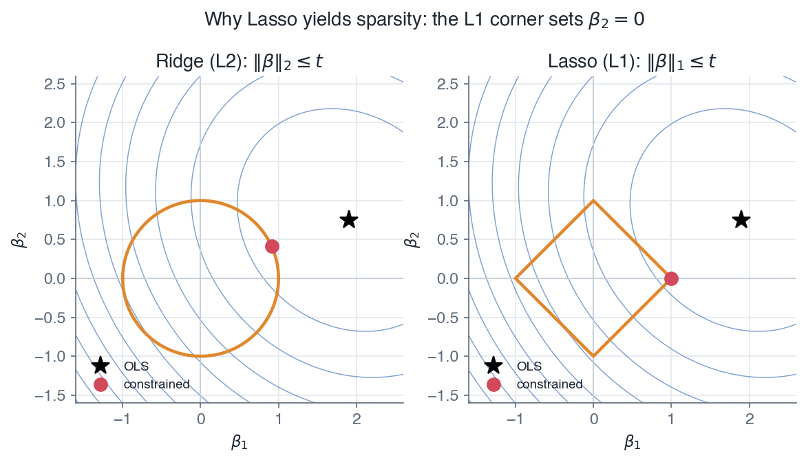
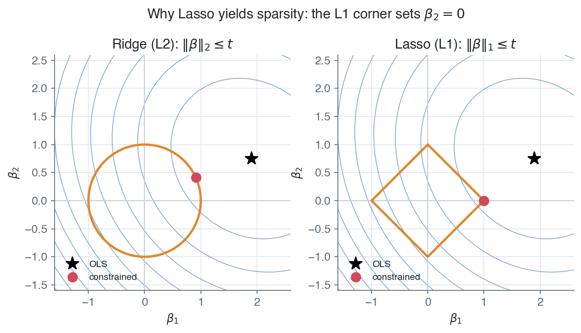
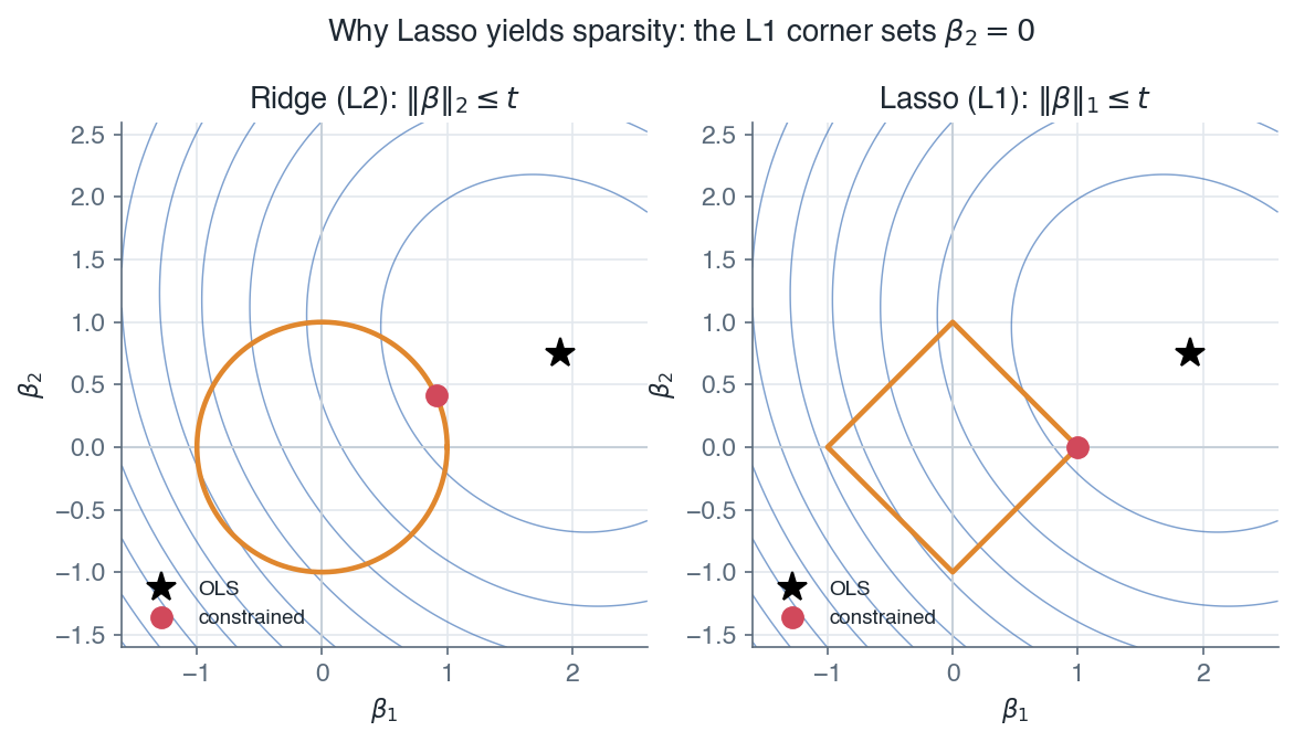
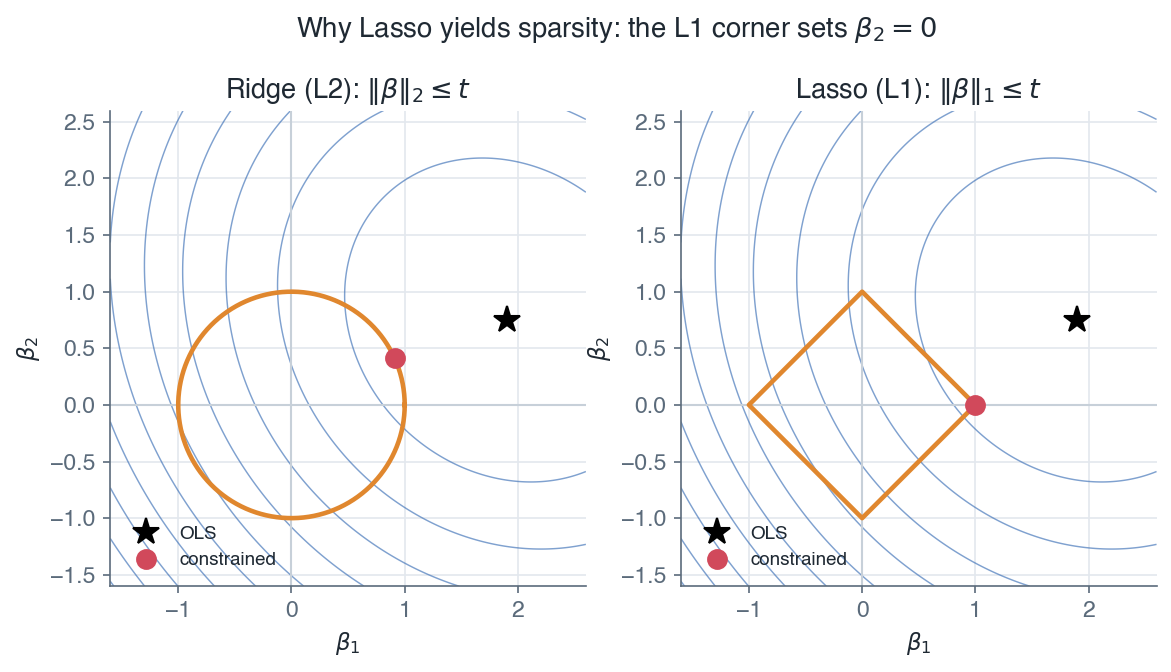
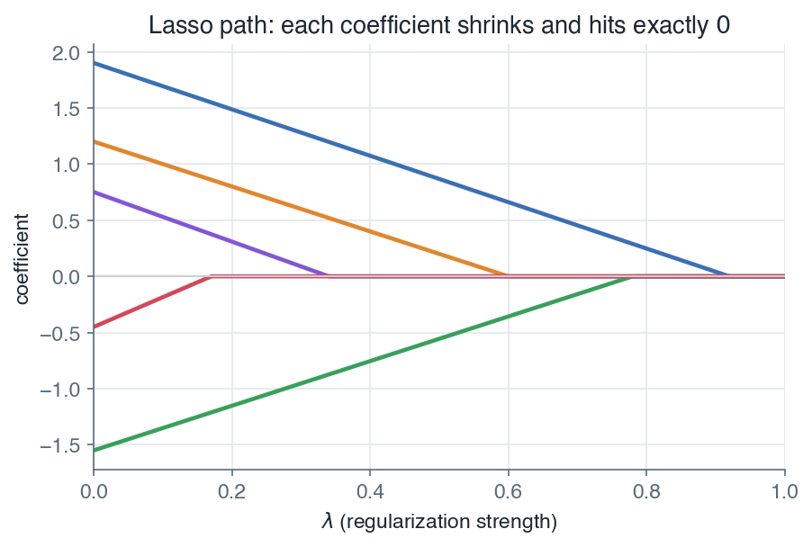
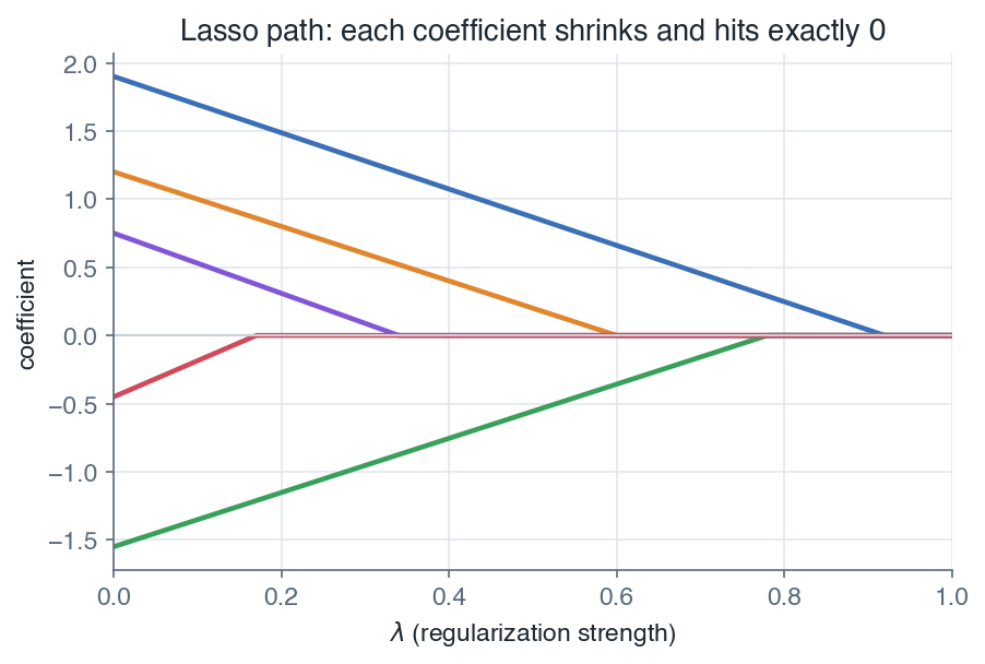
	This small change has a large consequence: the lasso drives some coefficients to exactly zero, so it performs variable selection while it fits. The reason is geometric. The constraint region $\|\beta\|_1 \le t$ is a diamond with corners on the axes, and the elliptical loss contours tend to first touch it at a corner, where one coordinate is zero.
-	
+	
	*The rounded L2 ball is touched off the axes, keeping every coefficient nonzero, while the L1 diamond is touched at a corner, setting a coefficient to exactly zero.*
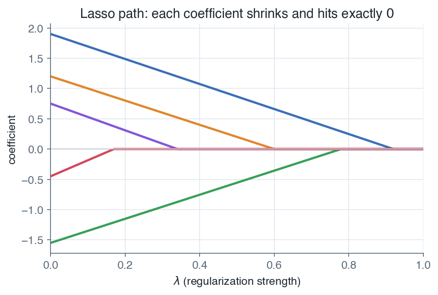
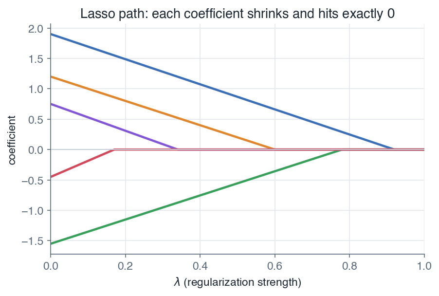
	As the penalty grows, more coefficients cross to zero, tracing the regularization path from the full model to the empty one.
-	
+	
	*Each coefficient shrinks as $\lambda$ increases and then hits exactly zero, so the lasso yields a compact, interpretable subset of regressors.*
-	## 5.4 Elastic net
+	## 7.4 Elastic net
	The elastic net blends the two penalties, keeping the lasso's selection while borrowing the ridge's stability with correlated regressors:
@@ 53,11 53,11 @@
	with $\alpha \in [0, 1]$ mixing selection ($\alpha = 1$, lasso) and shrinkage ($\alpha = 0$, ridge).
-	## 5.5 Choosing the penalty
+	## 7.5 Choosing the penalty
	The penalty $\lambda$ is a hyperparameter, so it is chosen by cross-validation from the [previous module](/en/Machine%20Learning/03%20Model%20evaluation%20and%20validation): fit over a grid of $\lambda$ values and keep the one with the lowest cross-validated error, or the largest $\lambda$ within one standard error of the best for a simpler model. Larger $\lambda$ means more shrinkage, more bias, and less variance.
-	## 5.6 The inference caveat
+	## 7.6 The inference caveat
	Prediction is not inference, and this is the point that is easy to miss. Suppose you select regressors with the lasso and then run ordinary least squares on the chosen subset and report textbook standard errors. Those standard errors are wrong. They ignore that the data was already used to pick the variables, so the confidence intervals are too narrow and the p-values are not valid, a form of the winner's curse. Three corrections are standard:
@@ 72,4 72,4 @@
	*With shrinkage and selection covered, the next module takes a different route to a good decision boundary, the maximum-margin classifier, before we turn to trees and ensembles.*
	---
-	Next: [Support Vector Machines](/en/Machine%20Learning/06%20Support%20Vector%20Machines) · [Course overview](/en/Machine%20Learning)
+	Next: [Support Vector Machines](/en/Machine%20Learning/08%20Support%20Vector%20Machines) · [Course overview](/en/Machine%20Learning)
en/Machine Learning/05 Regularization and high-dimensional inference/l1-l2-geometry.png .. en/Machine Learning/07 Regularization and high-dimensional inference/l1-l2-geometry.png
en/Machine Learning/05 Regularization and high-dimensional inference/regularization-path.png .. en/Machine Learning/07 Regularization and high-dimensional inference/regularization-path.png
en/Machine Learning/06 Support Vector Machines.md .. en/Machine Learning/08 Support Vector Machines.md
@@ 1,4 1,4 @@
-	# 6. Support Vector Machines
+	# 8. Support Vector Machines
	Support vector machines are large-margin linear classifiers. They pick the boundary that
	maximizes the distance to the nearest points, control overfitting with the hinge loss and a
@@ 11,11 11,11 @@
	- Define kernels, the kernel trick, and the Mercer condition.
	- Form the Lagrangian, derive the dual and KKT conditions, and define support vectors.
-	## 6.1 Optimal margin classifier
+	## 8.1 Optimal margin classifier
	Labels are $y \in \{-1,+1\}$, with weight vector $w \in \mathbb{R}^{n}$ and bias $b$.
-	### 6.1.1 Hypothesis and boundary
+	### 8.1.1 Hypothesis and boundary
	The hypothesis is defined as the sign of the raw score $z = w^T x - b$:
@@ 27,7 27,7 @@
	*Remark:* $w$ is orthogonal to the boundary, so it sets the orientation, and $b$ sets the offset.
-	### 6.1.2 Geometric margin
+	### 8.1.2 Geometric margin
	The geometric margin of example $i$ is defined as its signed distance to the boundary, made
	positive by the label:
@@ 40,7 40,7 @@
	*Remark:* dividing by $\lVert w \rVert$ makes the margin invariant to rescaling $(w,b)$, unlike
	the raw score $z$.
-	### 6.1.3 Hard-margin primal
+	### 8.1.3 Hard-margin primal
	Fixing the scale so the closest points satisfy $y^{(i)}(w^T x^{(i)} - b) = 1$, maximizing the
	margin is equivalent to minimizing $\lVert w \rVert^2$ subject to a unit functional margin:
@@ 52,15 52,15 @@
	*Remark:* it requires the data to be linearly separable. The next lesson relaxes that with slack
	variables.
-	
+	
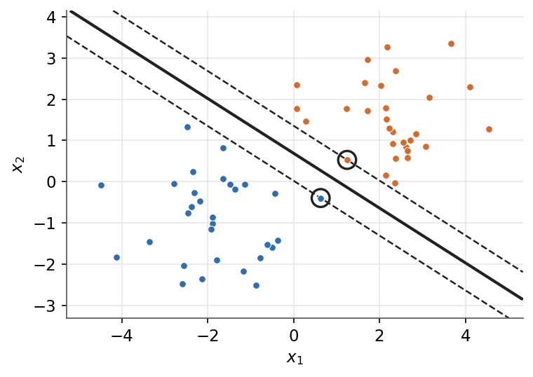
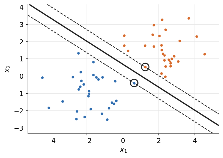
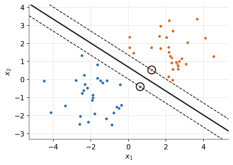
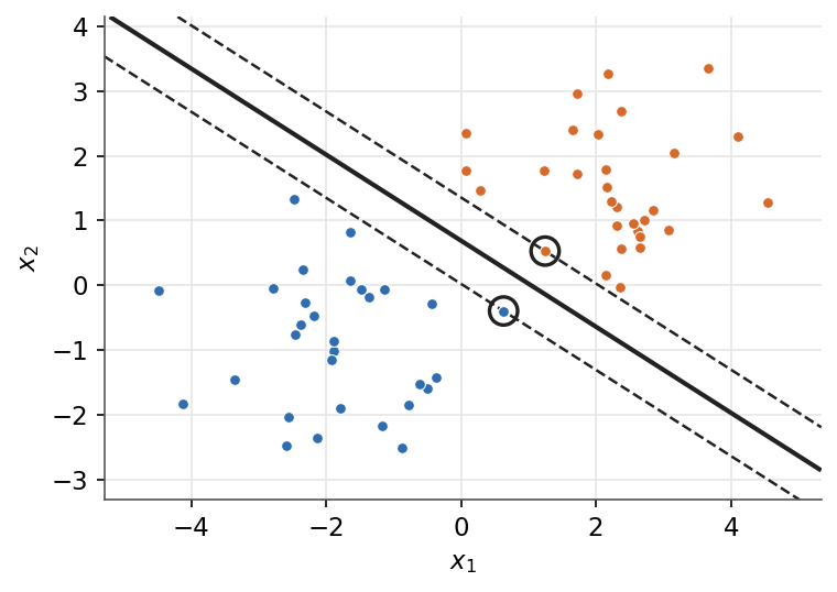
	*The optimal hyperplane (solid) maximizes the margin (dashed). Circled points are the support vectors.*
-	## 6.2 Hinge loss
+	## 8.2 Hinge loss
	The raw score is $z = w^T x - b$ and labels are $y \in \{-1,+1\}$.
-	### 6.2.1 Hinge loss
+	### 8.2.1 Hinge loss
	The hinge loss is defined as the amount by which the margin $yz$ falls short of $1$, clipped at zero:
@@ 72,7 72,7 @@
	*Remark:* the hinge loss is convex but not differentiable at $yz = 1$, so it is optimized with
	subgradients.
-	### 6.2.2 Soft-margin primal
+	### 8.2.2 Soft-margin primal
	Introduce a slack $\xi_i \ge 0$ per example to allow margin violations, penalized by $C > 0$:
@@ 86,7 86,7 @@
	This is regularization plus hinge loss: the $\tfrac{1}{2}\lVert w \rVert^2$ term widens the margin
	and the sum penalizes violations.
-	### 6.2.3 Role of $C$
+	### 8.2.3 Role of $C$
	| $C$ | Penalty on violations | Margin | Behaviour |
	| --- | --- | --- | --- |
@@ 95,9 95,9 @@
	*Remark:* as $C \to \infty$ no violation is tolerated, which recovers the hard-margin classifier.
-	## 6.3 Kernels
+	## 8.3 Kernels
-	### 6.3.1 Kernel definition
+	### 8.3.1 Kernel definition
	A kernel is defined as the inner product of a feature map $\phi$ applied to two inputs:
@@ 106,7 106,7 @@
	A valid kernel computes this inner product directly, so $\phi$ never has to be formed (it may even
	be infinite-dimensional).
-	### 6.3.2 Kernel trick
+	### 8.3.2 Kernel trick
	The SVM dual depends on the data only through inner products $\langle x^{(i)}, x^{(j)} \rangle$.
	The kernel trick replaces each inner product with a kernel:
@@ 120,7 120,7 @@
	$$\boxed{ K(x,z) = \exp\!\left( -\frac{\lVert x - z \rVert^2}{2\sigma^2} \right) }$$
-	### 6.3.3 Mercer condition
+	### 8.3.3 Mercer condition
	A function $K$ is a valid kernel if and only if, for every finite sample, its Gram matrix is
	symmetric positive semidefinite:
@@ 130,7 130,7 @@
	*Remark:* this is the Mercer condition. It guarantees a feature map $\phi$ exists, so the dual stays
	convex.
-	### 6.3.4 Common kernels
+	### 8.3.4 Common kernels
	| Kernel | $K(x,z)$ | Note |
	| --- | --- | --- |
@@ 141,13 141,13 @@
	*Remark:* a small $\sigma$ makes the RBF kernel very local, which can overfit. It trades off against
	$C$.
-	
+	
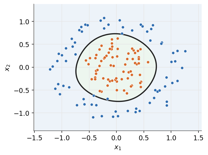
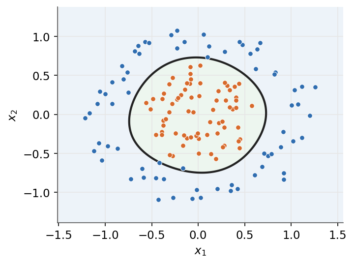
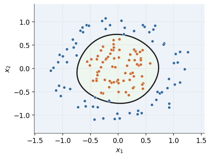
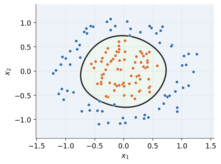
	*An RBF kernel separates classes that are not linearly separable, with a nonlinear boundary in the input space.*
-	## 6.4 Lagrangian and duality
+	## 8.4 Lagrangian and duality
-	### 6.4.1 Lagrangian
+	### 8.4.1 Lagrangian
	For a primal objective $f(w)$ with inequality constraints $g_i(w) \le 0$ and multipliers
	$\beta_i \ge 0$, the Lagrangian is defined as:
@@ 162,16 162,16 @@
	So the optimal $w$ is a linear combination of the training inputs weighted by $\beta_i y^{(i)}$.
-	### 6.4.2 Dual problem
+	### 8.4.2 Dual problem
	Substituting these back eliminates $w$ and $b$, leaving a problem in $\beta$ that depends on the
	data only through inner products:
	$$\boxed{ \max_{\beta} \ \sum_{i=1}^{m}\beta_i - \tfrac{1}{2}\sum_{i,j}\beta_i \beta_j\, y^{(i)} y^{(j)} \langle x^{(i)}, x^{(j)} \rangle \quad \text{s.t.} \quad \beta_i \ge 0, \ \ \sum_{i}\beta_i y^{(i)} = 0 }$$
-	The inner products are exactly where a kernel $K$ is substituted (see [Kernels](/en/Machine%20Learning/06%20Support%20Vector%20Machines#63-kernels)).
+	The inner products are exactly where a kernel $K$ is substituted (see [Kernels](/en/Machine%20Learning/08%20Support%20Vector%20Machines#83-kernels)).
-	### 6.4.3 KKT and support vectors
+	### 8.4.3 KKT and support vectors
	At the optimum, complementary slackness ties each multiplier to its constraint:
@@ 183,7 183,7 @@
	These are the points exactly on the margin. All others have $\beta_i = 0$ and do not affect $w$.
-	### 6.4.4 Kernelized decision
+	### 8.4.4 Kernelized decision
	Replacing the inner product by a kernel gives a decision rule expressed only through support vectors:
@@ 192,7 192,7 @@
	*Remark:* only support vectors ($\beta_i > 0$) contribute, so prediction cost scales with their
	count, not with $m$.
-	### 6.4.5 From primal to decision
+	### 8.4.5 From primal to decision
	```mermaid
	flowchart TD
@@ 212,4 212,4 @@
	*Support vector machines draw a single, possibly kernelized, boundary. The final part takes a different route: split the feature space with simple rules and combine many such models into an ensemble.*
	---
-	Next: [Decision trees and ensemble methods](/en/Machine%20Learning/07%20Decision%20trees%20and%20ensemble%20methods) · [Course overview](/en/Machine%20Learning)
+	Next: [Decision trees and ensemble methods](/en/Machine%20Learning/09%20Decision%20trees%20and%20ensemble%20methods) · [Course overview](/en/Machine%20Learning)
en/Machine Learning/06 Support Vector Machines/svm-kernel.png .. en/Machine Learning/08 Support Vector Machines/svm-kernel.png
en/Machine Learning/06 Support Vector Machines/svm-margin.png .. en/Machine Learning/08 Support Vector Machines/svm-margin.png
en/Machine Learning/07 Decision trees and ensemble methods.md .. en/Machine Learning/09 Decision trees and ensemble methods.md
@@ 1,4 1,4 @@
-	# 7. Decision trees and ensemble methods
+	# 9. Decision trees and ensemble methods
	Tree models partition the input space into axis-aligned regions and fit a constant per region, giving interpretable but high-variance predictors. Ensemble methods combine many trees: bagging and random forests average independently grown trees to cut variance, while boosting grows trees sequentially to cut bias.
@@ 9,9 9,9 @@
	- Estimate generalization error for free with out-of-bag samples.
	- Build a strong predictor as an additive sum of weak learners (AdaBoost, gradient boosting).
-	## 7.1 CART decision trees
+	## 9.1 CART decision trees
-	### 7.1.1 Tree as a partition
+	### 9.1.1 Tree as a partition
	A CART tree partitions the input space into $M$ disjoint regions $R_1,\dots,R_M$ (the leaves) and predicts a constant $c_m$ on each. The prediction is defined as
@@ 21,7 21,7 @@
	*Remark:* the regions are axis-aligned boxes, so the decision boundary is a staircase. A single tree has low bias but high variance.
-	### 7.1.2 Impurity and split selection
+	### 9.1.2 Impurity and split selection
	For a region with class proportions $\hat p_k$, impurity measures how mixed the labels are. The Gini index is defined as
@@ 44,7 44,7 @@
	*Remark:* the two criteria almost always pick the same split. Gini is the default in most implementations because it avoids the logarithm.
-	### 7.1.3 Regression trees
+	### 9.1.3 Regression trees
	For regression the leaf value is the mean of the targets in the region, defined as
@@ 52,7 52,7 @@
	and splits minimize the within-region squared error instead of a classification impurity.
-	### 7.1.4 Pruning
+	### 9.1.4 Pruning
	An unpruned tree fits the training set exactly and overfits. Cost-complexity pruning trades fit against tree size $|T|$ (the number of leaves) through a penalty $\alpha\ge0$:
@@ 68,13 68,13 @@
	B -->|"no"| E["leaf R2"]
	```
-	
+	
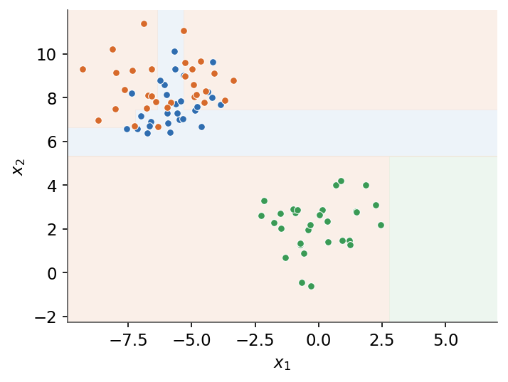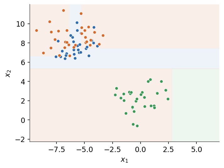
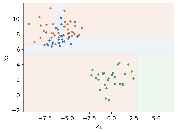
	*A tree carves the input space into axis-aligned regions, each with a constant prediction.*
-	## 7.2 Random forests
+	## 9.2 Random forests
-	### 7.2.1 Bagging
+	### 9.2.1 Bagging
	Bagging (bootstrap aggregating) trains $B$ trees on $B$ bootstrap resamples of the data and averages them. The bagged predictor is defined as
@@ 84,7 84,7 @@
	A bootstrap sample draws $N$ examples with replacement from $N$ examples. The probability that a given example is never drawn is $(1-\tfrac1N)^N\to e^{-1}\approx0.37$, so about 37% of the data is left out of each tree. These are its out-of-bag (OOB) examples.
-	### 7.2.2 Variance of an average
+	### 9.2.2 Variance of an average
	If the $B$ trees each have variance $\sigma^2$ and pairwise correlation $\rho$, the variance of their average is
@@ 92,7 92,7 @@
	The second term vanishes as $B$ grows, but the first, $\rho\sigma^2$, does not. Reducing the correlation $\rho$ between trees is therefore the key lever, and that is what random forests target.
-	### 7.2.3 Random forests
+	### 9.2.3 Random forests
	A random forest is bagging plus feature subsampling: at each split only a random subset of $m_{\text{try}}$ features is considered as split candidates. The usual choices are
@@ 122,13 122,13 @@
	T3 --> AGG
	```
-	
+	
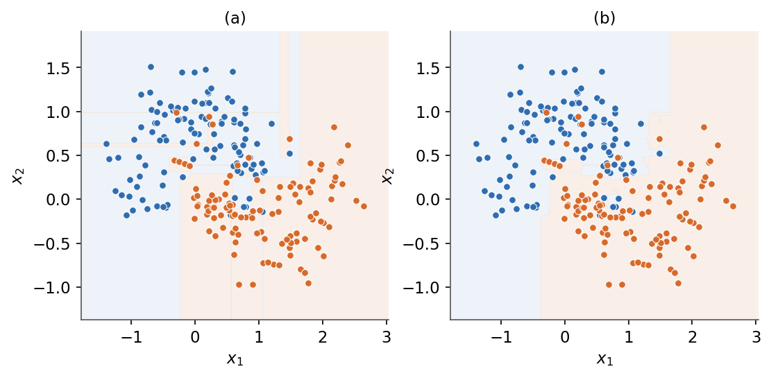
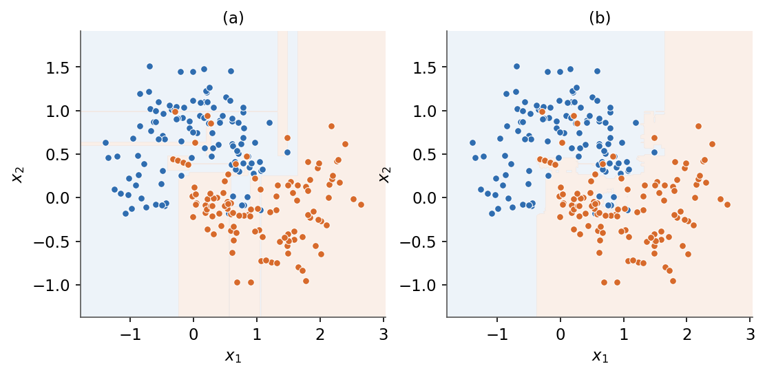
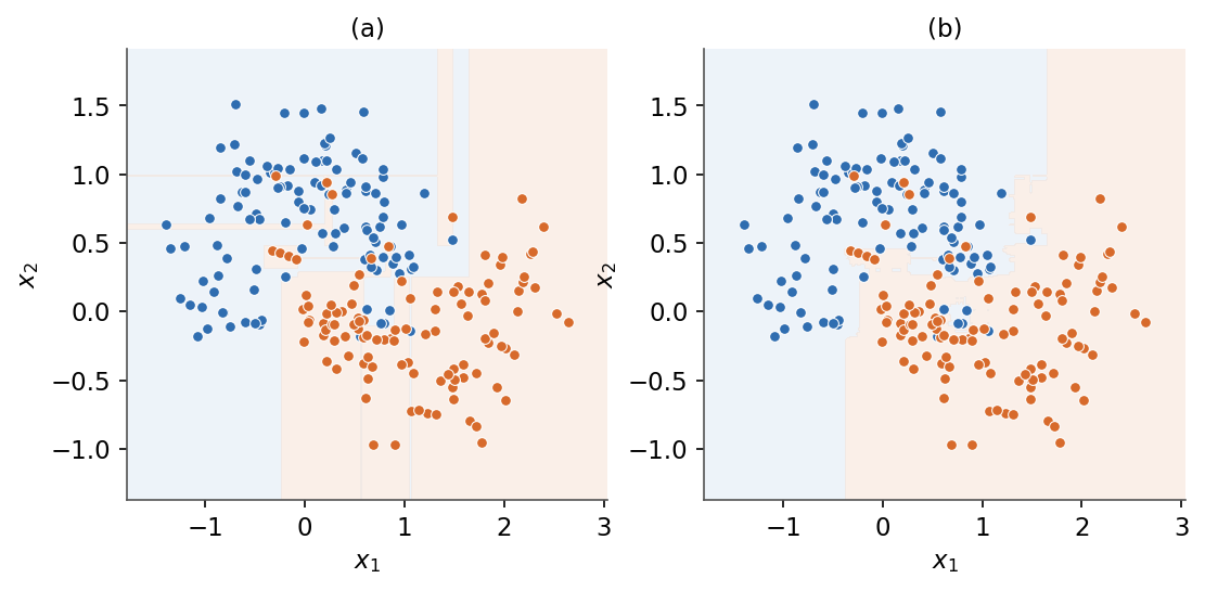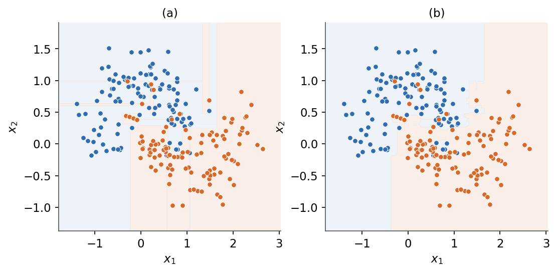
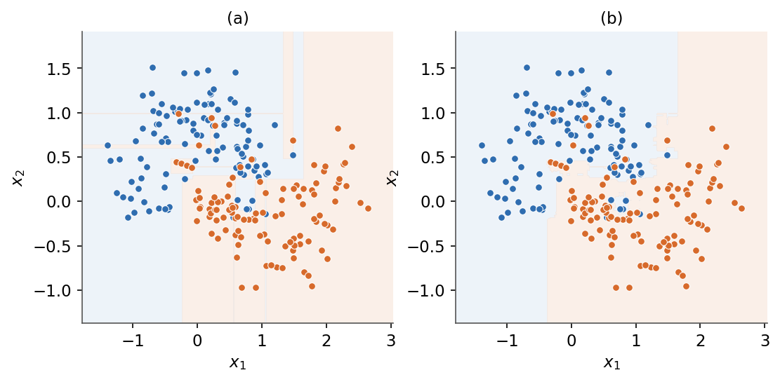
	*(a) A single deep tree overfits with a jagged boundary. (b) A random forest averages many trees for a smoother boundary.*
-	## 7.3 Boosting
+	## 9.3 Boosting
-	### 7.3.1 Additive model
+	### 9.3.1 Additive model
	Boosting builds a predictor as a weighted sum of $T$ weak learners $h_t$ (typically shallow trees), fitted one at a time. The additive model is defined as
@@ 136,7 136,7 @@
	Each stage corrects the errors of the running sum, so the ensemble is built sequentially and reduces bias rather than variance.
-	### 7.3.2 AdaBoost
+	### 9.3.2 AdaBoost
	With labels $y\in\{-1,+1\}$, AdaBoost keeps example weights $w^{(i)}$ that concentrate on the currently misclassified points. At round $t$ the weak learner has weighted error $\varepsilon_t$, and its coefficient is defined as
@@ 148,7 148,7 @@
	and renormalized. Misclassified examples ($y^{(i)}h_t(x^{(i)})<0$) gain weight, so the next learner focuses on them.
-	### 7.3.3 Gradient boosting
+	### 9.3.3 Gradient boosting
	Gradient boosting generalizes the idea to any differentiable loss $L$. At stage $t$ it fits the next learner to the negative gradient of the loss evaluated at the current model, the pseudo-residual defined as
en/Machine Learning/07 Decision trees and ensemble methods/forest-vs-tree.png .. en/Machine Learning/09 Decision trees and ensemble methods/forest-vs-tree.png
en/Machine Learning/07 Decision trees and ensemble methods/tree-boundary.png .. en/Machine Learning/09 Decision trees and ensemble methods/tree-boundary.png
/dev/null .. en/Mathematics.md
@@ 0,0 1,10 @@
+	# Mathematics
+
+	A short refresher of the mathematics the other courses build on: linear algebra, expectation and covariance, the multivariate Gaussian, and the Bayesian quantities (likelihood, prior, posterior, evidence).
+
+	## Syllabus
+
+	1. [Mathematical refresher](/en/Mathematics/01%20Mathematical%20refresher)
+
+	---
+	[Machine Learning](/en/Machine%20Learning) · [Home](/en)
/dev/null .. en/Mathematics/01 Mathematical refresher.md
@@ 0,0 1,79 @@
+	# 1. Mathematical refresher
+
+	This module gathers the mathematical tools the rest of the course leans on: a little linear algebra, the language of expectation and covariance, the multivariate Gaussian, and the four probability quantities (likelihood, prior, posterior, evidence) that the next module turns into a way of reasoning. It is a reference to return to, not a full treatment.
+
+	**Objectives**
+	- Recall the vector and matrix operations used throughout: dot product, matrix-vector product, transpose, inverse, and norm.
+	- Define expectation, variance, and covariance, and assemble the covariance matrix.
+	- Write the multivariate Gaussian density and read its shape from the covariance.
+	- Name the likelihood, prior, posterior, and evidence, and relate them by Bayes' rule.
+
+	## 1.1 Linear algebra
+
+	A feature vector lives in $\mathbb{R}^n$ and a dataset stacks such vectors into a matrix. The dot product of two vectors sums their elementwise products:
+
+	$$\boxed{ x^T y = \sum_{i=1}^{n} x_i\, y_i }$$
+
+	A matrix $A$ maps a vector by the matrix-vector product $Ax$, the transpose $A^T$ swaps rows and columns, and the inverse $A^{-1}$ (when it exists) undoes $A$, so $A^{-1}A = I$. The Euclidean norm measures length:
+
+	$$\boxed{ \lVert x \rVert_2 = \sqrt{x^T x} }$$
+
+	A square matrix is symmetric if $A = A^T$, and positive semidefinite if $x^T A x \ge 0$ for every $x$. Covariance matrices, which appear next, are always symmetric and positive semidefinite.
+
+	## 1.2 Expectation and variance
+
+	The expectation is the probability-weighted average of a random variable, a sum in the discrete case and an integral in the continuous one:
+
+	$$\boxed{ \mathbb{E}[X] = \sum_x x\, p(x) \qquad \mathbb{E}[X] = \int x\, p(x)\, dx }$$
+
+	Expectation is linear, $\mathbb{E}[aX + b] = a\,\mathbb{E}[X] + b$. The variance measures spread around the mean $\mu = \mathbb{E}[X]$:
+
+	$$\boxed{ \mathrm{Var}(X) = \mathbb{E}\!\left[(X - \mu)^2\right] = \mathbb{E}[X^2] - \mu^2 }$$
+
+	## 1.3 Covariance and the covariance matrix
+
+	Covariance measures how two variables move together:
+
+	$$\boxed{ \mathrm{Cov}(X, Y) = \mathbb{E}\!\left[(X - \mu_X)(Y - \mu_Y)\right] }$$
+
+	For a random vector $x \in \mathbb{R}^n$ with mean $\mu$, the covariance matrix collects every pairwise covariance:
+
+	$$\boxed{ \Sigma = \mathbb{E}\!\left[(x - \mu)(x - \mu)^T\right], \qquad \Sigma_{ij} = \mathrm{Cov}(x_i, x_j) }$$
+
+	Its diagonal holds the per-feature variances, it is symmetric, and it is positive semidefinite. Off-diagonal entries record correlation between features.
+
+	## 1.4 The multivariate Gaussian
+
+	The Gaussian is the default model for continuous noise and for smooth clouds of points. In $n$ dimensions it is parameterized by a mean vector $\mu$ and a covariance matrix $\Sigma$:
+
+	$$\boxed{ p(x) = \frac{1}{(2\pi)^{n/2}\,|\Sigma|^{1/2}} \exp\!\left(-\tfrac{1}{2}(x - \mu)^T \Sigma^{-1}(x - \mu)\right) }$$
+
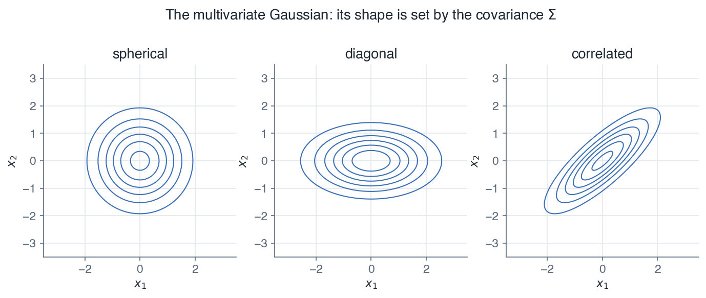
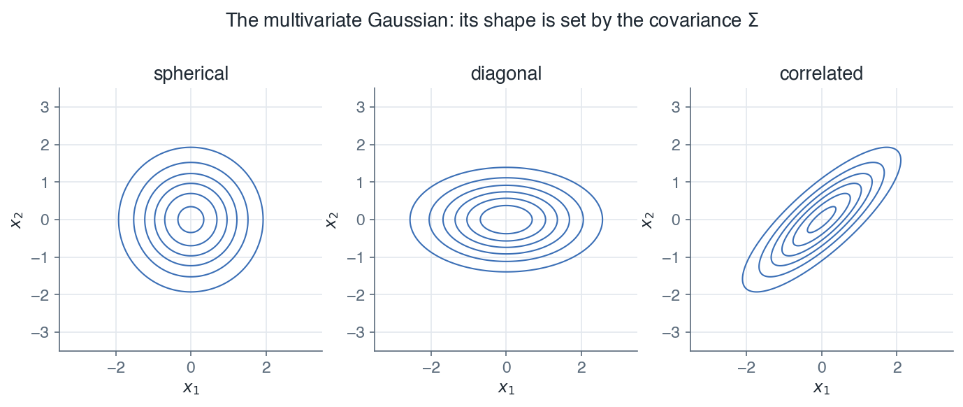
+	Its contours of equal density are ellipsoids centred at $\mu$, and the covariance $\Sigma$ sets their spread and orientation.
+
+	
+
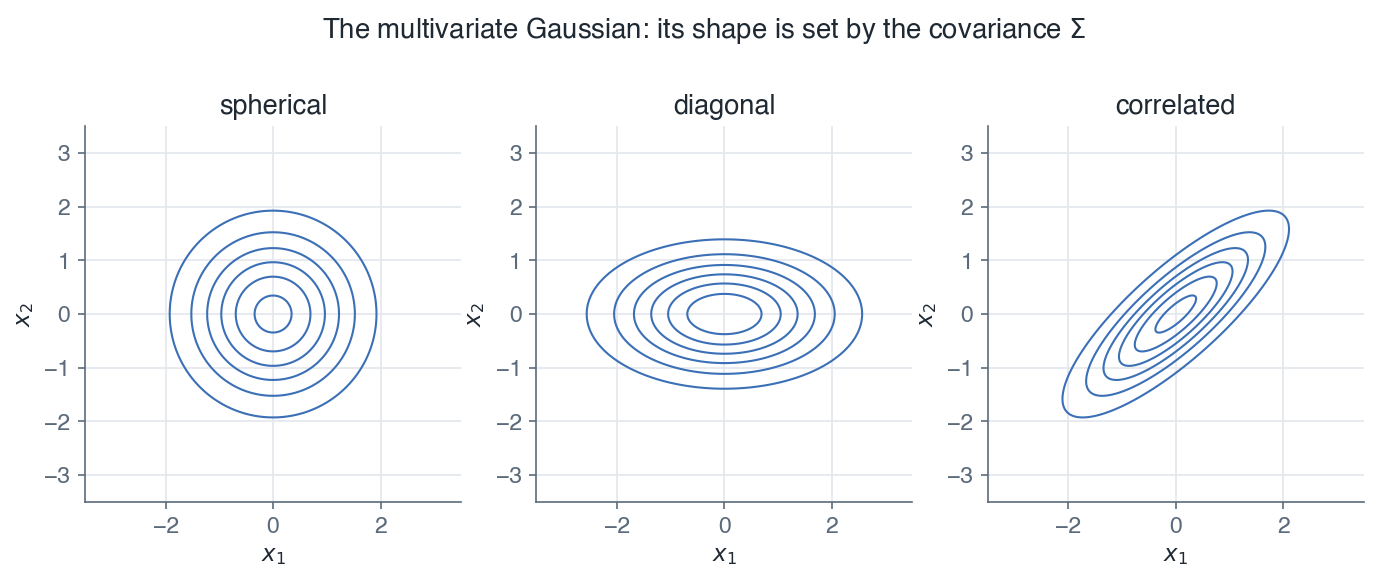+	*A spherical covariance gives circular contours, a diagonal one gives axis-aligned ellipses, and off-diagonal terms tilt them, encoding correlation between the features.*
+
+	*Remark:* the quadratic form $(x - \mu)^T \Sigma^{-1}(x - \mu)$ is the squared Mahalanobis distance, the natural distance once the data has a covariance structure.
+
+	## 1.5 Likelihood, prior, posterior, and evidence
+
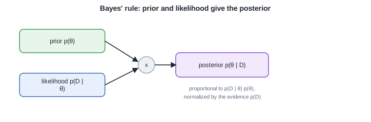
+	Almost every model in this course reasons about parameters $\theta$ given data $D$. Four quantities recur, and they are tied together by Bayes' rule:
+
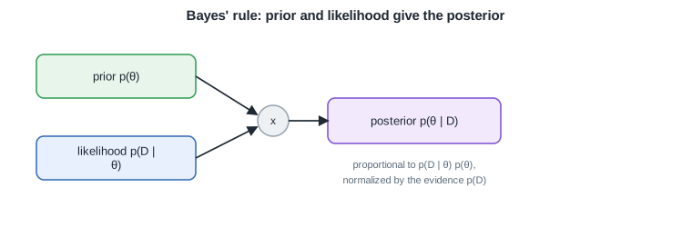
+	$$\boxed{ p(\theta \mid D) = \frac{p(D \mid \theta)\, p(\theta)}{p(D)} }$$
+
+	- The **likelihood** $p(D \mid \theta)$ is how probable the data is under a given $\theta$.
+	- The **prior** $p(\theta)$ is what we believed about $\theta$ before seeing the data.
+	- The **posterior** $p(\theta \mid D)$ is the updated belief after seeing it.
+	- The **evidence** $p(D) = \int p(D \mid \theta)\, p(\theta)\, d\theta$ normalizes the posterior so it integrates to one.
+
+	
+
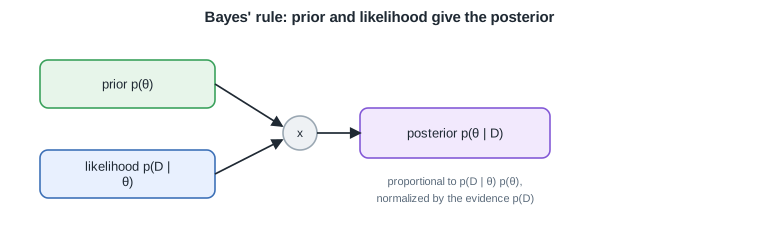+	*The posterior is proportional to the likelihood times the prior, divided by the evidence that makes it a proper distribution.*
+
+	*Remark:* the evidence is a constant with respect to $\theta$, so for many tasks it can be ignored and only the numerator $p(D \mid \theta)\, p(\theta)$ matters.
+
+	*These tools underpin the [Machine Learning](/en/Machine%20Learning) course, where probability, loss functions, and models are built on them.*
+
+	---
+	Next: [Course overview](/en/Mathematics)
/dev/null .. en/Mathematics/01 Mathematical refresher/bayes-rule.svg
@@ 0,0 1,1 @@
+	<svg xmlns="http://www.w3.org/2000/svg" viewBox="0 0 760 250" width="760" height="250" font-family="Helvetica, Arial, sans-serif"><defs><marker id="arrow" viewBox="0 0 10 10" refX="8.5" refY="5" markerWidth="7" markerHeight="7" orient="auto-start-reverse"><path d="M0 0L10 5L0 10z" fill="#1f2933"/></marker><marker id="arrowmuted" viewBox="0 0 10 10" refX="8.5" refY="5" markerWidth="7" markerHeight="7" orient="auto-start-reverse"><path d="M0 0L10 5L0 10z" fill="#5b6b7b"/></marker></defs><rect width="760" height="250" fill="#ffffff"/><text x="380.0" y="22.0" font-family="Helvetica, Arial, sans-serif" font-size="15" font-weight="600" fill="#1f2933" text-anchor="middle">Bayes&#x27; rule: prior and likelihood give the posterior</text><rect x="40.0" y="60.0" width="175.0" height="48.0" rx="8" fill="#e7f5ea" stroke="#38a05a" stroke-width="1.6"/><text x="127.5" y="88.4" font-family="Helvetica, Arial, sans-serif" font-size="13" fill="#1f2933" text-anchor="middle">prior p(θ)</text><rect x="40.0" y="150.0" width="175.0" height="48.0" rx="8" fill="#e8f0fe" stroke="#3b6fb6" stroke-width="1.6"/><text x="127.5" y="170.8" font-family="Helvetica, Arial, sans-serif" font-size="13" fill="#1f2933" text-anchor="middle">likelihood p(D |</text><text x="127.5" y="186.1" font-family="Helvetica, Arial, sans-serif" font-size="13" fill="#1f2933" text-anchor="middle">θ)</text><circle cx="300.0" cy="133.0" r="17.0" fill="#eef1f4" stroke="#9aa7b2" stroke-width="1.6"/><text x="300.0" y="137.1" font-family="Helvetica, Arial, sans-serif" font-size="12" fill="#1f2933" text-anchor="middle">x</text><line x1="215.0" y1="84.0" x2="282.0" y2="126.0" stroke="#1f2933" stroke-width="1.7" marker-end="url(#arrow)"/><line x1="215.0" y1="174.0" x2="282.0" y2="140.0" stroke="#1f2933" stroke-width="1.7" marker-end="url(#arrow)"/><rect x="360.0" y="108.0" width="190.0" height="50.0" rx="8" fill="#f2e9fd" stroke="#8257d6" stroke-width="1.6"/><text x="455.0" y="137.4" font-family="Helvetica, Arial, sans-serif" font-size="13" fill="#1f2933" text-anchor="middle">posterior p(θ | D)</text><line x1="317.0" y1="133.0" x2="360.0" y2="133.0" stroke="#1f2933" stroke-width="1.7" marker-end="url(#arrow)"/><text x="455.0" y="185.0" font-family="Helvetica, Arial, sans-serif" font-size="11" fill="#5b6b7b" text-anchor="middle">proportional to p(D | θ) p(θ),</text><text x="455.0" y="202.0" font-family="Helvetica, Arial, sans-serif" font-size="11" fill="#5b6b7b" text-anchor="middle">normalized by the evidence p(D)</text></svg>
\	No newline at end of file
/dev/null .. en/Mathematics/01 Mathematical refresher/multivariate-gaussian.png
fr.md ..
@@ 1,10 1,11 @@
	# Cours ML & MLOps
-	Trois cours sur le machine learning, le deep learning et la mise en production des modèles. Utilisez
-	les drapeaux en haut de la page pour changer de langue.
+	Quatre cours couvrant les mathématiques du machine learning, les méthodes de ML et de deep learning,
+	et la mise en production des modèles. Utilisez les drapeaux en haut de la page pour changer de langue.
	## Cours
+	- [Mathematics](/fr/Mathematics) : l'algèbre linéaire et les probabilités sur lesquelles reposent les cours.
	- [Machine Learning](/fr/Machine%20Learning) : les fondements du ML, des données aux modèles.
	- [Deep Learning](/fr/Deep%20Learning) : les réseaux de neurones, du perceptron aux transformeurs.
	- [MLOps](/fr/MLOps) : mettre les systèmes de ML en production et les maintenir.
fr/Deep Learning.md ..
@@ 2,7 2,7 @@
	Les réseaux de neurones, du simple perceptron aux transformeurs modernes : comment la profondeur, les bonnes fonctions d'activation et l'entraînement par gradient permettent à un modèle d'apprendre ses propres caractéristiques au lieu de les concevoir à la main.
-	**Prérequis :** le cours [Machine Learning](/fr/Machine%20Learning) (en particulier le perceptron dans [Modèles linéaires](/fr/Machine%20Learning/04%20Linear%20models)), Python de base, calcul différentiel et algèbre linéaire.
+	**Prérequis :** le cours [Machine Learning](/fr/Machine%20Learning) (en particulier le perceptron dans [Classification linéaire](/fr/Machine%20Learning/06%20Linear%20classification)), Python de base, calcul différentiel et algèbre linéaire.
	## Programme
fr/Deep Learning/01 Introduction.md ..
@@ 1,6 1,6 @@
	# 1. Introduction
-	Ce cours prolonge directement le cours de Machine Learning, qui concluait la partie [Modèles linéaires](/fr/Machine%20Learning/04%20Linear%20models) sur une remarque clé : un perceptron est une unité unique, et empilé en couches il devient un réseau de neurones. Cette leçon rend ce pont explicite. Elle rappelle ce qu'une seule unité peut faire, montre la tâche concrète (XOR) où une unité unique échoue, et fixe la notation utilisée dans tout le reste du cours.
+	Ce cours prolonge directement le cours de Machine Learning, qui concluait la partie [Classification linéaire](/fr/Machine%20Learning/06%20Linear%20classification) sur une remarque clé : un perceptron est une unité unique, et empilé en couches il devient un réseau de neurones. Cette leçon rend ce pont explicite. Elle rappelle ce qu'une seule unité peut faire, montre la tâche concrète (XOR) où une unité unique échoue, et fixe la notation utilisée dans tout le reste du cours.
	**Objectifs**
	- Rappeler le perceptron comme une unité unique avec une activation en marche d'escalier et une frontière linéaire.
fr/Machine Learning.md ..
@@ 2,17 2,19 @@
	Les fondements du machine learning : passer de données brutes à un modèle entraîné et évalué.
-	**Prérequis :** Python de base, notions d'algèbre linéaire et de statistiques.
+	**Prérequis :** Python de base et le cours [Mathematics](/fr/Mathematics) (algèbre linéaire, probabilités, statistiques).
	## Programme
	1. [Introduction](/fr/Machine%20Learning/01%20Introduction)
	2. [Concepts généraux](/fr/Machine%20Learning/02%20General%20concepts)
	3. [Évaluation et validation des modèles](/fr/Machine%20Learning/03%20Model%20evaluation%20and%20validation)
-	4. [Modèles linéaires](/fr/Machine%20Learning/04%20Linear%20models)
-	5. [Régularisation et inférence en grande dimension](/fr/Machine%20Learning/05%20Regularization%20and%20high-dimensional%20inference)
-	6. [Machines à vecteurs de support](/fr/Machine%20Learning/06%20Support%20Vector%20Machines)
-	7. [Arbres de décision et méthodes d'ensemble](/fr/Machine%20Learning/07%20Decision%20trees%20and%20ensemble%20methods)
+	4. [Formulation probabiliste](/fr/Machine%20Learning/04%20Probabilistic%20formulation)
+	5. [Régression linéaire](/fr/Machine%20Learning/05%20Linear%20regression)
+	6. [Classification linéaire](/fr/Machine%20Learning/06%20Linear%20classification)
+	7. [Régularisation et inférence en grande dimension](/fr/Machine%20Learning/07%20Regularization%20and%20high-dimensional%20inference)
+	8. [Machines à vecteurs de support](/fr/Machine%20Learning/08%20Support%20Vector%20Machines)
+	9. [Arbres de décision et méthodes d'ensemble](/fr/Machine%20Learning/09%20Decision%20trees%20and%20ensemble%20methods)
	---
	[MLOps](/fr/MLOps) · [Accueil](/fr)
fr/Machine Learning/03 Model evaluation and validation.md ..
@@ 70,4 70,4 @@
	*Une fois la généralisation mesurable, le module suivant ajuste nos premiers modèles, et celui d'après contrôle leur complexité par la régularisation, réglée précisément avec cette validation croisée.*
	---
-	Suivant : [Modèles linéaires](/fr/Machine%20Learning/04%20Linear%20models) · [Vue d'ensemble du cours](/fr/Machine%20Learning)
+	Suivant : [Formulation probabiliste](/fr/Machine%20Learning/04%20Probabilistic%20formulation) · [Vue d'ensemble du cours](/fr/Machine%20Learning)
fr/Machine Learning/04 Linear models.md .. /dev/null
@@ 1,193 0,0 @@
-	# 4. Modèles linéaires
-
-	Les modèles linéaires prédisent à partir d'un score linéaire $\theta^T x$. Ce module couvre la régression linéaire (cibles continues), la régression logistique (classification binaire) et le cadre des modèles linéaires généralisés qui unifie les deux via la famille exponentielle. Chaque modèle est ajusté par maximum de vraisemblance et partage la même mise à jour par gradient.
-
-	**Objectifs**
-	- Définir l'hypothèse linéaire et ajuster $\theta$ par la mise à jour LMS ou par l'équation normale en forme close.
-	- Comprendre pourquoi les moindres carrés sont l'estimation du maximum de vraisemblance sous bruit gaussien.
-	- Transformer le score linéaire en probabilité via la sigmoïde et l'ajuster par montée de gradient ou méthode de Newton.
-	- Classer avec le perceptron et savoir quand sa règle d'apprentissage converge.
-	- Reconnaître la forme de la famille exponentielle et construire un MLG à partir de ses trois hypothèses.
-	- Retrouver les régressions linéaire, logistique et softmax comme cas particuliers.
-
-	## 4.1 Régression linéaire
-
-	### 4.1.1 Hypothèse
-
-	L'hypothèse est linéaire en l'entrée augmentée $x \in \mathbb{R}^{n+1}$ avec $x_0 = 1$ et les paramètres $\theta \in \mathbb{R}^{n+1}$ :
-
-	$$\boxed{ h_\theta(x) = \theta^T x }$$
-
-	### 4.1.2 Fonction de coût
-
-	Le coût est défini comme la demi-somme des carrés des résidus sur les $m$ exemples :
-
-	$$\boxed{ J(\theta) = \tfrac{1}{2}\sum_{i=1}^{m}\left(h_\theta(x^{(i)}) - y^{(i)}\right)^2 }$$
-
-	### 4.1.3 Mise à jour LMS
-
-	La descente de gradient sur $J$ donne la mise à jour des moindres carrés moyens (Widrow-Hoff), appliquée par exemple $(x^{(i)}, y^{(i)})$ :
-
-	$$\boxed{ \theta_j \leftarrow \theta_j + \alpha\left(y^{(i)} - h_\theta(x^{(i)})\right)x_j^{(i)} }$$
-
-	avec un taux d'apprentissage $\alpha > 0$.
-
-	| variante | règle de mise à jour | par étape | à utiliser quand |
-	| --- | --- | --- | --- |
-	| GD par lots | somme sur les $m$ exemples | $O(mn)$ | $m$ petit à modéré |
-	| GD stochastique (SGD) | un exemple à la fois | $O(n)$ | $m$ grand, flux de données |
-
-	### 4.1.4 Équation normale
-
-	Annuler $\nabla_\theta J(\theta) = 0$ donne une solution en forme close à partir de la matrice de conception $X$ et du vecteur cible $y$ :
-
-	$$\boxed{ \theta = (X^T X)^{-1}X^T y }$$
-
-	*Remarque :* l'équation normale ne demande ni taux d'apprentissage ni itération, mais inverser $X^T X$ coûte $O(n^3)$, donc pour $n$ grand la mise à jour itérative LMS est préférée.
-
-	### 4.1.5 Interprétation probabiliste
-
-	Supposons $y^{(i)} = \theta^T x^{(i)} + \varepsilon^{(i)}$ avec un bruit gaussien i.i.d. $\varepsilon^{(i)} \sim \mathcal{N}(0, \sigma^2)$. Maximiser la log-vraisemblance revient alors à minimiser le coût des moindres carrés :
-
-	$$\boxed{ \arg\max_\theta \ell(\theta) = \arg\min_\theta J(\theta) }$$
-
-	*Remarque :* c'est pourquoi les moindres carrés sont un objectif fondé et pas seulement commode.
-
-	
-
-	*Les moindres carrés ajustent la droite qui minimise les résidus au carré (segments gris).*
-
-	## 4.2 Régression logistique
-
-	### 4.2.1 Sigmoïde
-
-	La fonction sigmoïde (logistique) comprime un score brut $z \in \mathbb{R}$ en une probabilité :
-
-	$$\boxed{ g(z) = \frac{1}{1 + e^{-z}} \in (0, 1) }$$
-
-	Sa dérivée a la forme commode $g'(z) = g(z)\left(1 - g(z)\right)$.
-
-	### 4.2.2 Modèle
-
-	L'hypothèse renvoie la probabilité de la classe positive, $\phi$ étant la probabilité prédite :
-
-	$$\boxed{ \phi = h_\theta(x) = g(\theta^T x) = p(y = 1 \mid x; \theta) }$$
-
-	Les étiquettes valent $y \in \{0, 1\}$, donc la loi conditionnelle est de Bernoulli :
-
-	$$\boxed{ p(y \mid x; \theta) = \phi^{y}(1 - \phi)^{1 - y} }$$
-
-	### 4.2.3 Log-vraisemblance
-
-	Sur $m$ exemples i.i.d. la log-vraisemblance est l'opposé de l'entropie croisée sommée sur les données :
-
-	$$\boxed{ \ell(\theta) = \sum_{i=1}^{m}\left[ y^{(i)}\log \phi^{(i)} + (1 - y^{(i)})\log(1 - \phi^{(i)}) \right] }$$
-
-	avec $\phi^{(i)} = h_\theta(x^{(i)})$.
-
-	### 4.2.4 Montée de gradient
-
-	Maximiser $\ell$ par montée de gradient donne la même forme que la mise à jour LMS :
-
-	$$\boxed{ \theta_j \leftarrow \theta_j + \alpha\left(y^{(i)} - h_\theta(x^{(i)})\right)x_j^{(i)} }$$
-
-	*Remarque :* la mise à jour a la même forme que la régression linéaire, bien que $h_\theta$ soit maintenant la sigmoïde. Ce n'est pas un hasard, les deux sont des modèles linéaires généralisés.
-
-	### 4.2.5 Méthode de Newton
-
-	La méthode de Newton converge plus vite près de l'optimum. En une dimension :
-
-	$$\boxed{ \theta \leftarrow \theta - \frac{\ell'(\theta)}{\ell''(\theta)} }$$
-
-	Dans le cas vectoriel elle utilise la hessienne $H$ de $\ell$ :
-
-	$$\boxed{ \theta \leftarrow \theta - H^{-1}\nabla_\theta \ell(\theta) }$$
-
-	*Remarque :* la régression logistique n'a pas de solution en forme close pour $\theta$, elle est donc toujours ajustée itérativement (montée de gradient ou Newton).
-
-	
-
-	*À gauche : la sigmoïde envoie les scores dans l'intervalle (0,1). À droite : la frontière de décision et la probabilité prédite.*
-
-	## 4.3 Perceptron
-
-	Le perceptron est le premier classifieur linéaire. Il conserve le score linéaire $\theta^T x$ de la régression logistique mais remplace la sigmoïde par un seuil dur, donc la sortie est une étiquette de classe et non une probabilité. Les étiquettes valent $y \in \{0, 1\}$.
-
-	### 4.3.1 Activation et hypothèse
-
-	L'activation est la fonction échelon :
-
-	$$\boxed{ g(z) = \begin{cases} 1 & \text{si } z \ge 0 \\ 0 & \text{sinon} \end{cases} }$$
-
-	et l'hypothèse l'applique au score linéaire :
-
-	$$\boxed{ h_\theta(x) = g(\theta^T x) }$$
-
-	### 4.3.2 Règle d'apprentissage
-
-	Le perceptron est entraîné en ligne, un exemple à la fois, et ne corrige $\theta$ que sur un point mal classé :
-
-	$$\boxed{ \theta_j \leftarrow \theta_j + \alpha\left(y^{(i)} - h_\theta(x^{(i)})\right)x_j^{(i)} }$$
-
-	*Remarque :* c'est la même forme que la mise à jour LMS et que la montée de gradient logistique. Seule l'activation $g$ change (identité, sigmoïde, échelon). Quand la prédiction est correcte, le facteur $y^{(i)} - h_\theta(x^{(i)})$ est nul, donc les points bien classés laissent $\theta$ inchangé.
-
-	
-
-	*Le perceptron trouve un hyperplan séparateur. Ce n'est pas nécessairement celui à marge maximale que choisira le SVM.*
-
-	### 4.3.3 Convergence
-
-	| données | comportement |
-	| --- | --- |
-	| linéairement séparables | converge en un nombre fini de mises à jour |
-	| non séparables | ne converge jamais, les poids oscillent |
-
-	*Remarque :* le perceptron s'arrête au premier hyperplan qui sépare les données, généralement pas celui à la marge la plus large. Cet écart motive la machine à vecteurs de support (qui maximise la marge) et, empilé en couches, le réseau de neurones (un perceptron est une unité).
-
-	## 4.4 Modèles linéaires généralisés
-
-	### 4.4.1 Famille exponentielle
-
-	Une distribution appartient à la famille exponentielle si sa densité s'écrit avec le paramètre naturel $\eta$, la statistique suffisante $T(y)$, la log-partition $a(\eta)$ et la mesure de base $b(y)$ :
-
-	$$\boxed{ p(y; \eta) = b(y)\exp\left(\eta\, T(y) - a(\eta)\right) }$$
-
-	### 4.4.2 Hypothèses du MLG
-
-	Un MLG repose sur trois choix. La réponse appartient à la famille exponentielle, le paramètre naturel est linéaire en l'entrée, et la prédiction est la statistique suffisante espérée :
-
-	$$\boxed{ \eta = \theta^T x }$$
-
-	$$\boxed{ h_\theta(x) = \mathbb{E}\left[T(y) \mid x; \theta\right] }$$
-
-	### 4.4.3 Tableau des familles
-
-	| Distribution | $\eta$ | $T(y)$ | $a(\eta)$ | $b(y)$ |
-	| --- | --- | --- | --- | --- |
-	| Bernoulli | $\log\dfrac{\phi}{1-\phi}$ | $y$ | $\log(1 + e^{\eta})$ | $1$ |
-	| Gaussienne ($\sigma^2 = 1$) | $\mu$ | $y$ | $\tfrac{1}{2}\eta^2$ | $\dfrac{1}{\sqrt{2\pi}}e^{-y^2/2}$ |
-	| Poisson | $\log\lambda$ | $y$ | $e^{\eta}$ | $\dfrac{1}{y!}$ |
-	| Géométrique | $\log(1-\phi)$ | $y$ | $\log\dfrac{e^{\eta}}{1 - e^{\eta}}$ | $1$ |
-
-	*Remarque :* pour la Bernoulli, $\eta$ est le log-rapport de cotes et son inverse est la sigmoïde, $\phi = g(\eta)$. C'est pourquoi la régression logistique a cette forme.
-
-	### 4.4.4 Régression softmax
-
-	Pour des étiquettes multiclasses $y \in \{1, \dots, k\}$ le MLG donne la régression softmax, avec un vecteur de paramètres $\theta_k$ par classe :
-
-	$$\boxed{ p(y = k \mid x; \theta) = \frac{\exp(\theta_k^T x)}{\sum_{j}\exp(\theta_j^T x)} }$$
-
-	### 4.4.5 Recette du MLG
-
-	```mermaid
-	graph TD
-	A["choisir une distribution de reponse"] --> B["l ecrire en forme de famille exponentielle"]
-	B --> C["poser le parametre naturel eta lineaire en x"]
-	C --> D["la prediction est la statistique suffisante esperee"]
-	D --> E["ajuster theta par maximum de vraisemblance"]
-	```
-
-	*Les modèles linéaires, y compris le perceptron, se contentent d'une frontière qui sépare les classes. La partie suivante cherche la meilleure : la machine à vecteurs de support maximise la marge.*
-
-	---
-	Suivant : [Régularisation et inférence en grande dimension](/fr/Machine%20Learning/05%20Regularization%20and%20high-dimensional%20inference) · [Vue d'ensemble du cours](/fr/Machine%20Learning)
/dev/null .. fr/Machine Learning/04 Probabilistic formulation.md
@@ 0,0 1,75 @@
+	# 4. Formulation probabiliste
+
+	La probabilité est le langage que le machine learning utilise pour traiter l'incertitude. Ce module énonce les règles pour les variables discrètes et continues, jette un premier regard sur la théorie de l'information, montre la manière bayésienne de transformer des probabilités en décisions, et définit les deux principes d'estimation auxquels le cours revient sans cesse : le maximum de vraisemblance et le maximum a posteriori.
+
+	**Objectifs**
+	- Énoncer les règles de la probabilité pour les variables discrètes et continues.
+	- Relier les probabilités conjointe, conditionnelle et marginale par les règles de la somme et du produit et par la règle de Bayes.
+	- Mesurer l'incertitude avec l'entropie, l'entropie croisée et la divergence de Kullback-Leibler.
+	- Prendre la décision qui minimise la perte espérée, et retrouver le classifieur du maximum a posteriori.
+	- Définir les estimateurs du maximum de vraisemblance et du maximum a posteriori.
+
+	## 4.1 Probabilité, discrète et continue
+
+	Une variable aléatoire prend des valeurs avec des probabilités qui sont positives et qui somment ou s'intègrent à un. Une variable discrète a une fonction de masse, une variable continue une densité de probabilité :
+
+	$$\boxed{ \sum_x p(x) = 1 \qquad \int p(x)\, dx = 1, \quad p(x) \ge 0 }$$
+
+	Pour une variable continue, la probabilité s'attache à des intervalles au moyen d'une intégrale, $P(a \le X \le b) = \int_a^b p(x)\, dx$, et non à des points isolés.
+
+	## 4.2 Conjointe, conditionnelle et Bayes
+
+	Deux variables ont une distribution conjointe $p(x, y)$. Sommer (ou intégrer) une variable donne la marginale, la règle de la somme, et la conjointe se factorise en une conditionnelle fois une marginale, la règle du produit :
+
+	$$\boxed{ p(x) = \sum_y p(x, y) \qquad p(x, y) = p(y \mid x)\, p(x) }$$
+
+	En réarrangeant la règle du produit dans les deux sens on obtient la règle de Bayes, qui inverse une conditionnelle :
+
+	$$\boxed{ p(y \mid x) = \frac{p(x \mid y)\, p(y)}{p(x)} }$$
+
+	Deux variables sont indépendantes quand la conjointe est le produit des marginales, $p(x, y) = p(x)\, p(y)$.
+
+	## 4.3 Un peu de théorie de l'information
+
+	L'entropie d'une distribution mesure son incertitude, le nombre moyen de bits nécessaires pour décrire une issue :
+
+	$$\boxed{ H(X) = -\sum_x p(x)\log p(x) }$$
+
+	
+
+	*Pour une variable à deux issues, l'entropie est maximale en $p = 0.5$, là où l'issue est la plus difficile à prévoir, et nulle quand une issue est certaine.*
+
+	L'entropie croisée mesure le coût d'utiliser un modèle $q$ quand la vérité est $p$, et la divergence de Kullback-Leibler mesure à quelle distance $q$ se trouve de $p$ :
+
+	$$\boxed{ H(p, q) = -\sum_x p(x)\log q(x) \qquad D_{\mathrm{KL}}(p \,\|\, q) = \sum_x p(x)\log\frac{p(x)}{q(x)} \ge 0 }$$
+
+	*Remarque :* minimiser l'entropie croisée entre les vraies étiquettes et les prédictions d'un modèle revient à maximiser la vraisemblance de ces étiquettes. C'est pourquoi les réseaux de classification minimisent l'entropie croisée, un fil repris dans les modules suivants.
+
+	## 4.4 Théorie de la décision bayésienne
+
+	Pour classer une entrée $x$, la règle bayésienne utilise l'a posteriori sur les classes. Sous la perte 0-1, la décision qui minimise la perte espérée est simplement la classe la plus probable, et comme l'a posteriori est proportionnel à la densité conditionnelle de classe fois l'a priori, on peut la calculer des deux façons :
+
+	$$\boxed{ \hat{y} = \arg\max_y \; p(y \mid x) = \arg\max_y \; p(x \mid y)\, p(y) }$$
+
+	
+
+	*Chaque classe apporte sa densité mise à l'échelle par son a priori, et la frontière de décision tombe là où les deux sont égales. De chaque côté, la classe au plus grand a posteriori l'emporte.*
+
+	*Remarque :* c'est le classifieur optimal, appelé classifieur de Bayes. Chaque méthode plus loin dans le cours est, en pratique, une tentative d'approcher ces a posteriori à partir des données.
+
+	## 4.5 Maximum de vraisemblance et maximum a posteriori
+
+	On connaît rarement la vraie distribution, on estime donc ses paramètres $\theta$ à partir des données. Le maximum de vraisemblance choisit le $\theta$ qui rend les données observées les plus probables, maximisé en général comme une somme de log-vraisemblances sur les $m$ exemples :
+
+	$$\boxed{ \theta_{\mathrm{MV}} = \arg\max_\theta \sum_{i=1}^{m} \log p(x^{(i)} \mid \theta) }$$
+
+	Le maximum a posteriori maximise plutôt l'a posteriori, qui multiplie la vraisemblance par un a priori sur $\theta$ :
+
+	$$\boxed{ \theta_{\mathrm{MAP}} = \arg\max_\theta \; p(D \mid \theta)\, p(\theta) }$$
+
+	*Remarque :* le maximum a posteriori est le maximum de vraisemblance augmenté d'un a priori. Un a priori gaussien sur $\theta$ devient une pénalité L2 et un a priori de Laplace une pénalité L1, ce qui est exactement la régularisation d'un module ultérieur. Avec beaucoup de données l'a priori s'efface et les deux estimateurs coïncident.
+
+	*Le module suivant transforme ces principes en fonctions de perte concrètes et en la descente de gradient qui les minimise.*
+
+	---
+	Suivant : [Régression linéaire](/fr/Machine%20Learning/05%20Linear%20regression) · [Vue d'ensemble du cours](/fr/Machine%20Learning)
/dev/null .. fr/Machine Learning/04 Probabilistic formulation/bayes-decision.png
/dev/null .. fr/Machine Learning/04 Probabilistic formulation/entropy.png
/dev/null .. fr/Machine Learning/05 Linear regression.md
@@ 0,0 1,62 @@
+	# 5. Régression linéaire
+
+	La régression linéaire prédit une cible continue à partir d'un score linéaire $\theta^T x$. Ce module la présente de façon probabiliste, en prolongeant le module [Formulation probabiliste](/fr/Machine%20Learning/04%20Probabilistic%20formulation) : le modèle (étendu aux caractéristiques polynomiales), l'ajustement par maximum de vraisemblance, qui se révèle être les moindres carrés ordinaires, et l'ajustement par maximum a posteriori, qui ajoute un a priori et donne un ajustement régularisé.
+
+	**Objectifs**
+	- Écrire le modèle de régression linéaire et polynomiale et l'ajuster par moindres carrés.
+	- Donner à la régression une formulation probabiliste avec un bruit gaussien.
+	- Voir que le maximum de vraisemblance sous ce modèle est exactement les moindres carrés.
+	- Ajouter un a priori et ajuster par maximum a posteriori, retrouvant un ajustement régularisé.
+
+	## 5.1 Le modèle linéaire et polynomial
+
+	L'hypothèse est linéaire en l'entrée augmentée $x \in \mathbb{R}^{n+1}$ avec $x_0 = 1$ et les paramètres $\theta$ :
+
+	$$\boxed{ h_\theta(x) = \theta^T x }$$
+
+	La régression polynomiale est le même modèle appliqué à une transformation des caractéristiques. Remplacer $x$ par $\phi(x) = (1, x, x^2, \dots, x^d)$ ajuste un polynôme de degré $d$ tout en restant linéaire en les paramètres :
+
+	$$\boxed{ h_\theta(x) = \theta^T \phi(x) = \sum_{j=0}^{d} \theta_j\, x^{j} }$$
+
+	donc tout ce qui suit s'applique tel quel une fois que la matrice de conception $X$ empile les entrées transformées $\phi(x^{(i)})$ sur ses lignes.
+
+	## 5.2 Moindres carrés
+
+	Le coût est la demi-somme des carrés des résidus sur les $m$ exemples :
+
+	$$\boxed{ J(\theta) = \tfrac{1}{2}\sum_{i=1}^{m}\left(h_\theta(x^{(i)}) - y^{(i)}\right)^2 }$$
+
+	Poser $\nabla_\theta J = 0$ donne l'équation normale sous forme close, et la descente de gradient donne la mise à jour itérative équivalente :
+
+	$$\boxed{ \theta = (X^T X)^{-1}X^T y \qquad \theta_j \leftarrow \theta_j + \alpha\left(y^{(i)} - h_\theta(x^{(i)})\right)x_j^{(i)} }$$
+
+	
+
+	*Les moindres carrés ajustent la courbe qui minimise les résidus au carré (segments gris).*
+
+	## 5.3 Formulation probabiliste : maximum de vraisemblance
+
+	Donnons aux données une histoire générative : chaque cible est la prédiction linéaire plus un bruit gaussien indépendant,
+
+	$$\boxed{ y^{(i)} = \theta^T x^{(i)} + \varepsilon^{(i)}, \quad \varepsilon^{(i)} \sim \mathcal{N}(0, \sigma^2) }$$
+
+	donc $p(y^{(i)} \mid x^{(i)}; \theta) = \mathcal{N}(\theta^T x^{(i)}, \sigma^2)$. Maximiser la log-vraisemblance sur les $m$ exemples i.i.d. élimine tout terme indépendant de $\theta$ et laisse le coût des moindres carrés :
+
+	$$\boxed{ \arg\max_\theta \ell(\theta) = \arg\min_\theta \sum_{i=1}^{m}\left(y^{(i)} - \theta^T x^{(i)}\right)^2 }$$
+
+	*Remarque :* c'est pourquoi les moindres carrés sont un objectif fondé et pas seulement commode. Les moindres carrés ordinaires sont l'estimation du maximum de vraisemblance sous un bruit gaussien, exactement le principe du maximum de vraisemblance du module précédent.
+
+	## 5.4 Maximum a posteriori
+
+	Le maximum de vraisemblance peut surapprendre, surtout à haut degré polynomial. Placer un a priori gaussien centré sur les paramètres, $\theta \sim \mathcal{N}(0, \tau^2 I)$, et maximiser l'a posteriori ajoute une pénalité sur leur taille :
+
+	$$\boxed{ \theta_{\mathrm{MAP}} = \arg\min_\theta \; \sum_{i=1}^{m}\left(y^{(i)} - \theta^T x^{(i)}\right)^2 + \lambda \lVert \theta \rVert_2^2, \quad \lambda = \frac{\sigma^2}{\tau^2} }$$
+
+	C'est la régression régularisée (ridge) : l'a priori gaussien devient une pénalité L2, exactement le lien a priori vers pénalité noté au module précédent.
+
+	*Remarque :* un a priori plus fort (petit $\tau$) signifie un $\lambda$ plus grand et un rétrécissement plus marqué vers zéro. Avec beaucoup de données, la vraisemblance domine l'a priori et l'ajustement du maximum a posteriori se rapproche de celui du maximum de vraisemblance. Choisir le degré $d$ et la pénalité $\lambda$ est un problème de sélection de modèle, réglé par la validation croisée du [module d'évaluation](/fr/Machine%20Learning/03%20Model%20evaluation%20and%20validation), et approfondi dans le [module de régularisation](/fr/Machine%20Learning/07%20Regularization%20and%20high-dimensional%20inference).
+
+	*Le même score linéaire, passé dans une fonction de compression au lieu d'être lu directement, transforme la régression en classification, le sujet du module suivant.*
+
+	---
+	Suivant : [Classification linéaire](/fr/Machine%20Learning/06%20Linear%20classification) · [Vue d'ensemble du cours](/fr/Machine%20Learning)
fr/Machine Learning/04 Linear models/linear-regression.png .. fr/Machine Learning/05 Linear regression/linear-regression.png
/dev/null .. fr/Machine Learning/06 Linear classification.md
@@ 0,0 1,83 @@
+	# 6. Classification linéaire
+
+	La classification prédit une étiquette discrète à partir du même score linéaire $\theta^T x$. Ce module part de l'idée de traiter la classification comme une régression, puis construit les deux classifieurs linéaires classiques : le perceptron, binaire et multiclasse, et la régression logistique, binaire avec la sigmoïde et multiclasse avec la softmax, tous entraînés par descente de gradient sur l'entropie croisée.
+
+	**Objectifs**
+	- Voir pourquoi régresser directement les étiquettes est un mauvais classifieur, et comment une fonction de compression y remédie.
+	- Classer avec le perceptron, binaire et multiclasse, et savoir quand il converge.
+	- Ajuster la régression logistique binaire avec la sigmoïde et l'entropie croisée.
+	- Étendre à plusieurs classes avec la softmax, et relier la sigmoïde et la softmax.
+	- Entraîner ces modèles par descente de gradient.
+
+	## 6.1 La classification comme un problème de régression
+
+	On pourrait ajuster les moindres carrés directement aux étiquettes $y \in \{0, 1\}$, mais la sortie linéaire est non bornée, se laisse tirer par les valeurs aberrantes, et ne se lit pas comme une probabilité. La solution est de garder le score linéaire et de le passer dans une fonction de compression qui l'envoie vers une classe ou une probabilité. Le reste du module présente deux choix de cette fonction.
+
+	## 6.2 Le perceptron
+
+	### 6.2.1 Perceptron binaire
+
+	Le perceptron passe le score dans un échelon dur, si bien que la sortie est une étiquette de classe :
+
+	$$\boxed{ h_\theta(x) = g(\theta^T x), \quad g(z) = \begin{cases} 1 & \text{si } z \ge 0 \\ 0 & \text{sinon} \end{cases} }$$
+
+	Il est entraîné en ligne, corrigeant $\theta$ seulement sur un point mal classé :
+
+	$$\boxed{ \theta_j \leftarrow \theta_j + \alpha\left(y^{(i)} - h_\theta(x^{(i)})\right)x_j^{(i)} }$$
+
+	
+
+	*Le perceptron trouve un hyperplan séparateur, pas nécessairement celui de marge maximale que la machine à vecteurs de support choisira.*
+
+	### 6.2.2 Perceptron multiclasse
+
+	Avec $k$ classes, on garde un vecteur de poids $\theta_c$ par classe et on prédit celle au plus fort score. Sur une erreur, on récompense la vraie classe et on pénalise la classe prédite :
+
+	$$\boxed{ \hat{y} = \arg\max_c \theta_c^T x, \qquad \theta_{y} \mathrel{+}= \alpha x, \quad \theta_{\hat{y}} \mathrel{-}= \alpha x }$$
+
+	### 6.2.3 Convergence
+
+	Si les données sont linéairement séparables, le perceptron converge en un nombre fini de mises à jour, sinon les poids oscillent indéfiniment.
+
+	*Remarque :* le perceptron s'arrête au premier hyperplan séparateur, ce qui motive la machine à vecteurs de support (marge la plus large) et, empilé en couches, le réseau de neurones. Un perceptron est une unité unique, et empilé en couches il devient un réseau de neurones, le point de départ du cours de Deep Learning.
+
+	## 6.3 Régression logistique, binaire
+
+	La régression logistique remplace l'échelon dur par la sigmoïde lisse, si bien que la sortie est la probabilité de la classe positive :
+
+	$$\boxed{ \phi = p(y = 1 \mid x; \theta) = g(\theta^T x) = \frac{1}{1 + e^{-\theta^T x}} }$$
+
+	Elle est ajustée en minimisant l'entropie croisée, la log-vraisemblance négative des étiquettes de Bernoulli :
+
+	$$\boxed{ L(\theta) = -\sum_{i=1}^{m}\left[ y^{(i)}\log \phi^{(i)} + (1 - y^{(i)})\log(1 - \phi^{(i)}) \right] }$$
+
+	
+
+	*À gauche : la sigmoïde envoie tout score dans l'intervalle (0, 1). À droite : la frontière de décision et la probabilité prédite.*
+
+	## 6.4 Régression logistique, multiclasse
+
+	Pour $k$ classes, la sigmoïde se généralise en la softmax, un vecteur de poids par classe, normalisé en une distribution :
+
+	$$\boxed{ p(y = c \mid x; \theta) = \frac{\exp(\theta_c^T x)}{\sum_{j=1}^{k}\exp(\theta_j^T x)} }$$
+
+	entraînée par l'entropie croisée catégorielle $L = -\sum_i \log p(y^{(i)} \mid x^{(i)})$.
+
+	| | sigmoïde | softmax |
+	| --- | --- | --- |
+	| classes | 2 | $k$ |
+	| sortie | une probabilité $\phi$ | une distribution sur $k$ classes |
+	| relation | la softmax à $k = 2$ se réduit à la sigmoïde | généralise la sigmoïde |
+
+	## 6.5 Descente de gradient
+
+	Les deux modèles sont ajustés par descente de gradient sur l'entropie croisée. Le gradient prend la même forme épurée que la mise à jour des moindres carrés, le résidu fois l'entrée :
+
+	$$\boxed{ \theta_j \leftarrow \theta_j - \alpha \sum_{i=1}^{m}\left(\phi^{(i)} - y^{(i)}\right)x_j^{(i)} }$$
+
+	*Remarque :* le perceptron, la régression linéaire et la régression logistique partagent une seule mise à jour, le résidu fois l'entrée. Seule l'activation diffère (échelon, identité, sigmoïde ou softmax). Le cours de Deep Learning reprend précisément ce fil, en empilant de telles unités en couches.
+
+	*Les modèles linéaires étant couverts, le module suivant contrôle leur complexité : la régularisation et l'inférence quand les régresseurs sont nombreux.*
+
+	---
+	Suivant : [Régularisation et inférence en grande dimension](/fr/Machine%20Learning/07%20Regularization%20and%20high-dimensional%20inference) · [Vue d'ensemble du cours](/fr/Machine%20Learning)
fr/Machine Learning/04 Linear models/logistic-regression.png .. fr/Machine Learning/06 Linear classification/logistic-regression.png
fr/Machine Learning/04 Linear models/perceptron.png .. fr/Machine Learning/06 Linear classification/perceptron.png
fr/Machine Learning/05 Regularization and high-dimensional inference.md .. fr/Machine Learning/07 Regularization and high-dimensional inference.md
@@ 1,8 1,8 @@
-	# 5. Régularisation et inférence en grande dimension
+	# 7. Régularisation et inférence en grande dimension
	On n'a souvent pas une poignée de régresseurs propres. Il peut y avoir de nombreux prédicteurs candidats, parfois plus que d'observations, et ils sont corrélés. Les moindres carrés ordinaires surapprennent ou s'effondrent dans ce régime. La régularisation les dompte en rétrécissant les coefficients, et c'est là que la régression régularisée rejoint le plus directement la statistique classique. Elle s'accompagne d'un avertissement : sélectionner des variables puis faire de l'inférence sur les mêmes données invalide les écarts-types classiques, ce qui compte dès que l'objectif est une estimation causale plutôt qu'une prédiction.
-	Dans tout ce module, on note les coefficients de régression $\beta$, les paramètres $\theta$ du modèle linéaire du [module précédent](/fr/Machine%20Learning/04%20Linear%20models).
+	Dans tout ce module, on note les coefficients de régression $\beta$, les paramètres $\theta$ du modèle linéaire du [module de régression linéaire](/fr/Machine%20Learning/05%20Linear%20regression).
	**Objectifs**
	- Voir pourquoi les moindres carrés ordinaires échouent avec de nombreux régresseurs corrélés.
@@ 11,11 11,11 @@
	- Choisir la pénalité $\lambda$ par validation croisée.
	- Reconnaître pourquoi l'inférence naïve après sélection est invalide, et connaître les corrections standard.
-	## 5.1 Pourquoi régulariser
+	## 7.1 Pourquoi régulariser
	Quand le nombre de régresseurs $p$ est grand par rapport à la taille d'échantillon $n$, l'ajustement par moindres carrés poursuit le bruit et ses coefficients ont une variance énorme. Avec des régresseurs corrélés, la matrice $X^T X$ est presque singulière, donc de petites variations des données font osciller fortement les estimations, et quand $p > n$ elle est singulière et les MCO n'ont aucune solution unique. La régularisation accepte un peu de biais en échange d'une forte réduction de variance, le compromis vu dans [Concepts généraux](/fr/Machine%20Learning/02%20General%20concepts).
-	## 5.2 Régression ridge (L2)
+	## 7.2 Régression ridge (L2)
	Ridge ajoute une pénalité en norme au carré sur les coefficients à l'objectif des moindres carrés :
@@ 27,7 27,7 @@
	Ridge rétrécit tous les coefficients doucement vers zéro mais ne les annule jamais exactement, elle stabilise donc plutôt qu'elle ne sélectionne.
-	## 5.3 Régression lasso (L1)
+	## 7.3 Régression lasso (L1)
	Le lasso remplace la pénalité au carré par une pénalité en valeur absolue :
@@ 35,17 35,17 @@
	Ce petit changement a une grande conséquence : le lasso met certains coefficients exactement à zéro, il effectue donc une sélection de variables tout en ajustant. La raison est géométrique. La région de contrainte $\|\beta\|_1 \le t$ est un losange dont les coins sont sur les axes, et les contours elliptiques de la perte tendent à la toucher d'abord en un coin, où une coordonnée est nulle.
-	
+	
	*La boule L2 arrondie est touchée hors des axes, gardant chaque coefficient non nul, tandis que le losange L1 est touché en un coin, mettant un coefficient exactement à zéro.*
	À mesure que la pénalité grandit, davantage de coefficients passent à zéro, traçant le chemin de régularisation du modèle complet jusqu'au modèle vide.
-	
+	
	*Chaque coefficient rétrécit quand $\lambda$ augmente puis atteint exactement zéro, si bien que le lasso fournit un sous-ensemble compact et interprétable de régresseurs.*
-	## 5.4 Elastic net
+	## 7.4 Elastic net
	L'elastic net mêle les deux pénalités, gardant la sélection du lasso tout en empruntant la stabilité de ridge face aux régresseurs corrélés :
@@ 53,11 53,11 @@
	avec $\alpha \in [0, 1]$ dosant la sélection ($\alpha = 1$, lasso) et le rétrécissement ($\alpha = 0$, ridge).
-	## 5.5 Choisir la pénalité
+	## 7.5 Choisir la pénalité
	La pénalité $\lambda$ est un hyperparamètre, on la choisit donc par validation croisée, vue au [module précédent](/fr/Machine%20Learning/03%20Model%20evaluation%20and%20validation) : on ajuste sur une grille de valeurs de $\lambda$ et on garde celle dont l'erreur validée est la plus faible, ou le plus grand $\lambda$ à un écart-type du meilleur pour un modèle plus simple. Un $\lambda$ plus grand signifie plus de rétrécissement, plus de biais et moins de variance.
-	## 5.6 La mise en garde sur l'inférence
+	## 7.6 La mise en garde sur l'inférence
	Prédire n'est pas inférer, et c'est le point qu'il est facile de manquer. Supposons que vous sélectionniez des régresseurs par lasso, puis que vous fassiez des moindres carrés ordinaires sur le sous-ensemble retenu en rapportant les écarts-types des manuels. Ces écarts-types sont faux. Ils ignorent que les données ont déjà servi à choisir les variables, donc les intervalles de confiance sont trop étroits et les p-valeurs ne sont pas valides, une forme de la malédiction du vainqueur. Trois corrections sont standard :
@@ 72,4 72,4 @@
	*Une fois le rétrécissement et la sélection couverts, le module suivant emprunte une autre voie vers une bonne frontière de décision, le classifieur à marge maximale, avant d'aborder les arbres et les ensembles.*
	---
-	Suivant : [Machines à vecteurs de support](/fr/Machine%20Learning/06%20Support%20Vector%20Machines) · [Vue d'ensemble du cours](/fr/Machine%20Learning)
+	Suivant : [Machines à vecteurs de support](/fr/Machine%20Learning/08%20Support%20Vector%20Machines) · [Vue d'ensemble du cours](/fr/Machine%20Learning)
fr/Machine Learning/05 Regularization and high-dimensional inference/l1-l2-geometry.png .. fr/Machine Learning/07 Regularization and high-dimensional inference/l1-l2-geometry.png
fr/Machine Learning/05 Regularization and high-dimensional inference/regularization-path.png .. fr/Machine Learning/07 Regularization and high-dimensional inference/regularization-path.png
fr/Machine Learning/06 Support Vector Machines.md .. fr/Machine Learning/08 Support Vector Machines.md
@@ 1,4 1,4 @@
-	# 6. Machines à vecteurs de support
+	# 8. Machines à vecteurs de support
	Les machines à vecteurs de support sont des classifieurs linéaires à grande marge. Elles
	choisissent la frontière qui maximise la distance aux points les plus proches, contrôlent le
@@ 12,11 12,11 @@
	- Définir les noyaux, l'astuce du noyau et la condition de Mercer.
	- Former le lagrangien, dériver le dual et les conditions KKT, et définir les vecteurs de support.
-	## 6.1 Classifieur à marge optimale
+	## 8.1 Classifieur à marge optimale
	Les étiquettes valent $y \in \{-1,+1\}$, avec un vecteur de poids $w \in \mathbb{R}^{n}$ et un biais $b$.
-	### 6.1.1 Hypothèse et frontière
+	### 8.1.1 Hypothèse et frontière
	L'hypothèse est définie comme le signe du score brut $z = w^T x - b$ :
@@ 28,7 28,7 @@
	*Remarque :* $w$ est orthogonal à la frontière, il en fixe donc l'orientation, et $b$ fixe le décalage.
-	### 6.1.2 Marge géométrique
+	### 8.1.2 Marge géométrique
	La marge géométrique de l'exemple $i$ est définie comme sa distance signée à la frontière, rendue
	positive par l'étiquette :
@@ 41,7 41,7 @@
	*Remarque :* diviser par $\lVert w \rVert$ rend la marge invariante au rééchelonnement de $(w,b)$,
	contrairement au score brut $z$.
-	### 6.1.3 Primal à marge dure
+	### 8.1.3 Primal à marge dure
	En fixant l'échelle pour que les points les plus proches vérifient $y^{(i)}(w^T x^{(i)} - b) = 1$,
	maximiser la marge équivaut à minimiser $\lVert w \rVert^2$ sous une marge fonctionnelle unitaire :
@@ 53,15 53,15 @@
	*Remarque :* il exige des données linéairement séparables. La leçon suivante assouplit cela avec
	des variables d'écart.
-	
+	
	*L'hyperplan optimal (trait plein) maximise la marge (pointillés). Les points entourés sont les vecteurs de support.*
-	## 6.2 Perte charnière
+	## 8.2 Perte charnière
	Le score brut est $z = w^T x - b$ et les étiquettes valent $y \in \{-1,+1\}$.
-	### 6.2.1 Perte charnière
+	### 8.2.1 Perte charnière
	La perte charnière est définie comme l'écart par lequel la marge $yz$ tombe sous $1$, tronqué à zéro :
@@ 73,7 73,7 @@
	*Remarque :* la perte charnière est convexe mais non dérivable en $yz = 1$, on l'optimise donc
	avec des sous-gradients.
-	### 6.2.2 Primal à marge souple
+	### 8.2.2 Primal à marge souple
	On introduit un écart $\xi_i \ge 0$ par exemple pour autoriser les violations de marge, pénalisé
	par $C > 0$ :
@@ 88,7 88,7 @@
	C'est de la régularisation plus une perte charnière : le terme $\tfrac{1}{2}\lVert w \rVert^2$
	élargit la marge et la somme pénalise les violations.
-	### 6.2.3 Rôle de $C$
+	### 8.2.3 Rôle de $C$
	| $C$ | Pénalité des violations | Marge | Comportement |
	| --- | --- | --- | --- |
@@ 98,9 98,9 @@
	*Remarque :* quand $C \to \infty$ aucune violation n'est tolérée, ce qui redonne le classifieur à
	marge dure.
-	## 6.3 Noyaux
+	## 8.3 Noyaux
-	### 6.3.1 Définition d'un noyau
+	### 8.3.1 Définition d'un noyau
	Un noyau est défini comme le produit scalaire d'une application de caractéristiques $\phi$
	appliquée à deux entrées :
@@ 110,7 110,7 @@
	Un noyau valide calcule ce produit scalaire directement, donc $\phi$ n'a jamais à être formée
	(elle peut même être de dimension infinie).
-	### 6.3.2 Astuce du noyau
+	### 8.3.2 Astuce du noyau
	Le dual du SVM ne dépend des données qu'à travers des produits scalaires
	$\langle x^{(i)}, x^{(j)} \rangle$. L'astuce du noyau remplace chaque produit scalaire par un noyau :
@@ 124,7 124,7 @@
	$$\boxed{ K(x,z) = \exp\!\left( -\frac{\lVert x - z \rVert^2}{2\sigma^2} \right) }$$
-	### 6.3.3 Condition de Mercer
+	### 8.3.3 Condition de Mercer
	Une fonction $K$ est un noyau valide si et seulement si, pour tout échantillon fini, sa matrice de
	Gram est symétrique semi-définie positive :
@@ 134,7 134,7 @@
	*Remarque :* c'est la condition de Mercer. Elle garantit l'existence d'une application $\phi$, donc
	le dual reste convexe.
-	### 6.3.4 Noyaux usuels
+	### 8.3.4 Noyaux usuels
	| Noyau | $K(x,z)$ | Note |
	| --- | --- | --- |
@@ 145,13 145,13 @@
	*Remarque :* un petit $\sigma$ rend le noyau RBF très local, ce qui peut surapprendre. Il se règle
	en compromis avec $C$.
-	
+	
	*Un noyau RBF sépare des classes non linéairement séparables, par une frontière non linéaire dans l'espace d'entrée.*
-	## 6.4 Lagrangien et dualité
+	## 8.4 Lagrangien et dualité
-	### 6.4.1 Lagrangien
+	### 8.4.1 Lagrangien
	Pour un objectif primal $f(w)$ avec contraintes d'inégalité $g_i(w) \le 0$ et multiplicateurs
	$\beta_i \ge 0$, le lagrangien est défini comme :
@@ 167,16 167,16 @@
	Le $w$ optimal est donc une combinaison linéaire des entrées d'apprentissage pondérées par
	$\beta_i y^{(i)}$.
-	### 6.4.2 Problème dual
+	### 8.4.2 Problème dual
	En réinjectant ces relations, on élimine $w$ et $b$, ce qui laisse un problème en $\beta$ ne
	dépendant des données qu'à travers des produits scalaires :
	$$\boxed{ \max_{\beta} \ \sum_{i=1}^{m}\beta_i - \tfrac{1}{2}\sum_{i,j}\beta_i \beta_j\, y^{(i)} y^{(j)} \langle x^{(i)}, x^{(j)} \rangle \quad \text{s.c.} \quad \beta_i \ge 0, \ \ \sum_{i}\beta_i y^{(i)} = 0 }$$
-	Les produits scalaires sont exactement l'endroit où l'on substitue un noyau $K$ (voir [Noyaux](/fr/Machine%20Learning/06%20Support%20Vector%20Machines#63-noyaux)).
+	Les produits scalaires sont exactement l'endroit où l'on substitue un noyau $K$ (voir [Noyaux](/fr/Machine%20Learning/08%20Support%20Vector%20Machines#83-noyaux)).
-	### 6.4.3 KKT et vecteurs de support
+	### 8.4.3 KKT et vecteurs de support
	À l'optimum, l'écart complémentaire lie chaque multiplicateur à sa contrainte :
@@ 189,7 189,7 @@
	Ce sont les points exactement sur la marge. Tous les autres ont $\beta_i = 0$ et n'influencent pas
	$w$.
-	### 6.4.4 Décision à noyau
+	### 8.4.4 Décision à noyau
	Remplacer le produit scalaire par un noyau donne une règle de décision exprimée uniquement à
	travers les vecteurs de support :
@@ 199,7 199,7 @@
	*Remarque :* seuls les vecteurs de support ($\beta_i > 0$) contribuent, donc le coût de prédiction
	croît avec leur nombre, pas avec $m$.
-	### 6.4.5 Du primal à la décision
+	### 8.4.5 Du primal à la décision
	```mermaid
	flowchart TD
@@ 219,4 219,4 @@
	*Les machines à vecteurs de support tracent une seule frontière, éventuellement à noyau. La dernière partie suit une autre voie : découper l'espace des variables par des règles simples et combiner de nombreux modèles en un ensemble.*
	---
-	Suivant : [Arbres de décision et méthodes d'ensemble](/fr/Machine%20Learning/07%20Decision%20trees%20and%20ensemble%20methods) · [Vue d'ensemble du cours](/fr/Machine%20Learning)
+	Suivant : [Arbres de décision et méthodes d'ensemble](/fr/Machine%20Learning/09%20Decision%20trees%20and%20ensemble%20methods) · [Vue d'ensemble du cours](/fr/Machine%20Learning)
fr/Machine Learning/06 Support Vector Machines/svm-kernel.png .. fr/Machine Learning/08 Support Vector Machines/svm-kernel.png
fr/Machine Learning/06 Support Vector Machines/svm-margin.png .. fr/Machine Learning/08 Support Vector Machines/svm-margin.png
fr/Machine Learning/07 Decision trees and ensemble methods.md .. fr/Machine Learning/09 Decision trees and ensemble methods.md
@@ 1,4 1,4 @@
-	# 7. Arbres de décision et méthodes d'ensemble
+	# 9. Arbres de décision et méthodes d'ensemble
	Les modèles d'arbre partitionnent l'espace d'entrée en régions alignées sur les axes et ajustent une constante par région, ce qui donne des prédicteurs interprétables mais à forte variance. Les méthodes d'ensemble combinent plusieurs arbres : le bagging et les forêts aléatoires moyennent des arbres construits indépendamment pour réduire la variance, tandis que le boosting construit les arbres de façon séquentielle pour réduire le biais.
@@ 9,9 9,9 @@
	- Estimer gratuitement l'erreur de généralisation avec les échantillons hors-sac.
	- Construire un prédicteur fort comme somme additive d'apprenants faibles (AdaBoost, gradient boosting).
-	## 7.1 Arbres de décision CART
+	## 9.1 Arbres de décision CART
-	### 7.1.1 L'arbre comme partition
+	### 9.1.1 L'arbre comme partition
	Un arbre CART partitionne l'espace d'entrée en $M$ régions disjointes $R_1,\dots,R_M$ (les feuilles) et prédit une constante $c_m$ sur chacune. La prédiction est définie par
@@ 21,7 21,7 @@
	*Remarque :* les régions sont des boîtes alignées sur les axes, donc la frontière de décision est en escalier. Un arbre seul a un faible biais mais une forte variance.
-	### 7.1.2 Impureté et choix de la coupure
+	### 9.1.2 Impureté et choix de la coupure
	Pour une région de proportions de classes $\hat p_k$, l'impureté mesure le mélange des étiquettes. L'indice de Gini est défini par
@@ 44,7 44,7 @@
	*Remarque :* les deux critères choisissent presque toujours la même coupure. Gini est le défaut de la plupart des implémentations car il évite le logarithme.
-	### 7.1.3 Arbres de régression
+	### 9.1.3 Arbres de régression
	En régression, la valeur de la feuille est la moyenne des cibles dans la région, définie par
@@ 52,7 52,7 @@
	et les coupures minimisent l'erreur quadratique intra-région plutôt qu'une impureté de classification.
-	### 7.1.4 Élagage
+	### 9.1.4 Élagage
	Un arbre non élagué ajuste exactement l'ensemble d'entraînement et surapprend. L'élagage à complexité coûteuse arbitre entre l'ajustement et la taille de l'arbre $|T|$ (le nombre de feuilles) via une pénalité $\alpha\ge0$ :
@@ 68,13 68,13 @@
	B -->|"non"| E["feuille R2"]
	```
-	
+	
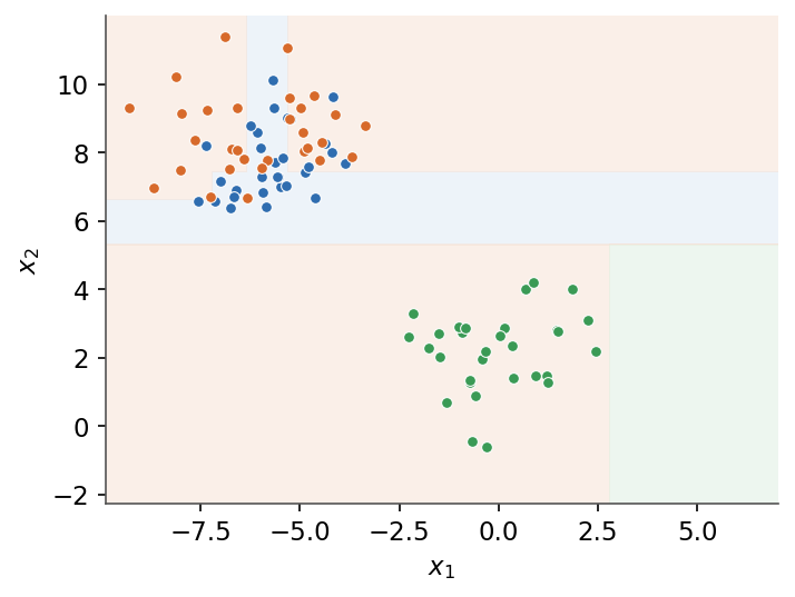	*Un arbre découpe l'espace en régions alignées sur les axes, chacune à prédiction constante.*
-	## 7.2 Forêts aléatoires
+	## 9.2 Forêts aléatoires
-	### 7.2.1 Bagging
+	### 9.2.1 Bagging
	Le bagging (bootstrap aggregating) entraîne $B$ arbres sur $B$ rééchantillons bootstrap des données et les moyenne. Le prédicteur agrégé est défini par
@@ 84,7 84,7 @@
	Un échantillon bootstrap tire $N$ exemples avec remise parmi $N$ exemples. La probabilité qu'un exemple donné ne soit jamais tiré vaut $(1-\tfrac1N)^N\to e^{-1}\approx0{,}37$, donc environ 37 % des données restent hors de chaque arbre. Ce sont ses exemples hors-sac (OOB).
-	### 7.2.2 Variance d'une moyenne
+	### 9.2.2 Variance d'une moyenne
	Si les $B$ arbres ont chacun une variance $\sigma^2$ et une corrélation deux à deux $\rho$, la variance de leur moyenne vaut
@@ 92,7 92,7 @@
	Le second terme s'annule quand $B$ croît, mais le premier, $\rho\sigma^2$, persiste. Réduire la corrélation $\rho$ entre les arbres est donc le levier clé, et c'est précisément ce que visent les forêts aléatoires.
-	### 7.2.3 Forêts aléatoires
+	### 9.2.3 Forêts aléatoires
	Une forêt aléatoire est du bagging avec sous-échantillonnage des variables : à chaque coupure, seul un sous-ensemble aléatoire de $m_{\text{try}}$ variables est considéré comme candidat. Les choix usuels sont
@@ 122,13 122,13 @@
	T3 --> AGG
	```
-	
+	
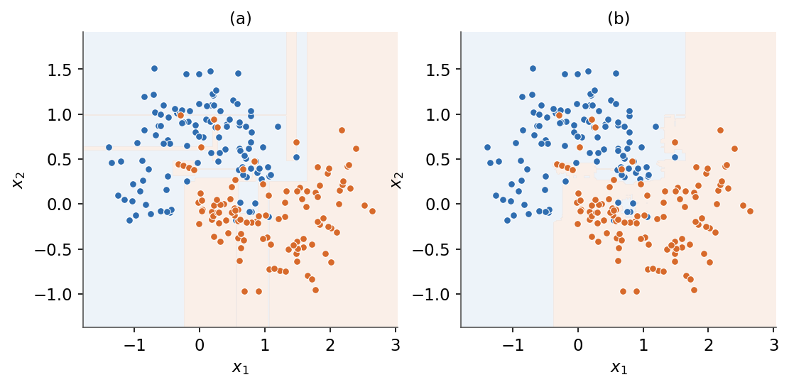	*(a) Un arbre profond seul surajuste avec une frontière en escalier. (b) Une forêt aléatoire moyenne de nombreux arbres pour une frontière plus lisse.*
-	## 7.3 Boosting
+	## 9.3 Boosting
-	### 7.3.1 Modèle additif
+	### 9.3.1 Modèle additif
	Le boosting construit un prédicteur comme une somme pondérée de $T$ apprenants faibles $h_t$ (typiquement des arbres peu profonds), ajustés un à un. Le modèle additif est défini par
@@ 136,7 136,7 @@
	Chaque étape corrige les erreurs de la somme courante, donc l'ensemble est construit de façon séquentielle et réduit le biais plutôt que la variance.
-	### 7.3.2 AdaBoost
+	### 9.3.2 AdaBoost
	Avec des étiquettes $y\in\{-1,+1\}$, AdaBoost conserve des poids d'exemples $w^{(i)}$ qui se concentrent sur les points actuellement mal classés. Au tour $t$, l'apprenant faible a une erreur pondérée $\varepsilon_t$, et son coefficient est défini par
@@ 148,7 148,7 @@
	puis renormalisés. Les exemples mal classés ($y^{(i)}h_t(x^{(i)})<0$) gagnent du poids, donc l'apprenant suivant se concentre sur eux.
-	### 7.3.3 Gradient boosting
+	### 9.3.3 Gradient boosting
	Le gradient boosting généralise l'idée à toute perte différentiable $L$. À l'étape $t$, il ajuste l'apprenant suivant sur l'opposé du gradient de la perte évalué au modèle courant, le pseudo-résidu défini par
fr/Machine Learning/07 Decision trees and ensemble methods/forest-vs-tree.png .. fr/Machine Learning/09 Decision trees and ensemble methods/forest-vs-tree.png
fr/Machine Learning/07 Decision trees and ensemble methods/tree-boundary.png .. fr/Machine Learning/09 Decision trees and ensemble methods/tree-boundary.png
/dev/null .. fr/Mathematics.md
@@ 0,0 1,10 @@
+	# Mathematics
+
+	Un bref rappel des mathématiques sur lesquelles reposent les autres cours : algèbre linéaire, espérance et covariance, gaussienne multivariée, et les quantités bayésiennes (vraisemblance, a priori, a posteriori, évidence).
+
+	## Programme
+
+	1. [Rappels mathématiques](/fr/Mathematics/01%20Mathematical%20refresher)
+
+	---
+	[Machine Learning](/fr/Machine%20Learning) · [Accueil](/fr)
/dev/null .. fr/Mathematics/01 Mathematical refresher.md
@@ 0,0 1,79 @@
+	# 1. Rappels mathématiques
+
+	Ce module rassemble les outils mathématiques sur lesquels s'appuie le reste du cours : un peu d'algèbre linéaire, le langage de l'espérance et de la covariance, la gaussienne multivariée, et les quatre quantités probabilistes (vraisemblance, a priori, a posteriori, évidence) que le module suivant transforme en une manière de raisonner. C'est une référence à consulter, pas un traitement complet.
+
+	**Objectifs**
+	- Rappeler les opérations sur vecteurs et matrices utilisées partout : produit scalaire, produit matrice-vecteur, transposée, inverse et norme.
+	- Définir l'espérance, la variance et la covariance, et assembler la matrice de covariance.
+	- Écrire la densité de la gaussienne multivariée et lire sa forme à partir de la covariance.
+	- Nommer la vraisemblance, l'a priori, l'a posteriori et l'évidence, et les relier par la règle de Bayes.
+
+	## 1.1 Algèbre linéaire
+
+	Un vecteur de caractéristiques vit dans $\mathbb{R}^n$ et un jeu de données empile de tels vecteurs dans une matrice. Le produit scalaire de deux vecteurs somme leurs produits terme à terme :
+
+	$$\boxed{ x^T y = \sum_{i=1}^{n} x_i\, y_i }$$
+
+	Une matrice $A$ transforme un vecteur par le produit matrice-vecteur $Ax$, la transposée $A^T$ échange lignes et colonnes, et l'inverse $A^{-1}$ (quand elle existe) annule $A$, donc $A^{-1}A = I$. La norme euclidienne mesure la longueur :
+
+	$$\boxed{ \lVert x \rVert_2 = \sqrt{x^T x} }$$
+
+	Une matrice carrée est symétrique si $A = A^T$, et semi-définie positive si $x^T A x \ge 0$ pour tout $x$. Les matrices de covariance, qui apparaissent juste après, sont toujours symétriques et semi-définies positives.
+
+	## 1.2 Espérance et variance
+
+	L'espérance est la moyenne pondérée par les probabilités d'une variable aléatoire, une somme dans le cas discret et une intégrale dans le cas continu :
+
+	$$\boxed{ \mathbb{E}[X] = \sum_x x\, p(x) \qquad \mathbb{E}[X] = \int x\, p(x)\, dx }$$
+
+	L'espérance est linéaire, $\mathbb{E}[aX + b] = a\,\mathbb{E}[X] + b$. La variance mesure la dispersion autour de la moyenne $\mu = \mathbb{E}[X]$ :
+
+	$$\boxed{ \mathrm{Var}(X) = \mathbb{E}\!\left[(X - \mu)^2\right] = \mathbb{E}[X^2] - \mu^2 }$$
+
+	## 1.3 Covariance et matrice de covariance
+
+	La covariance mesure comment deux variables évoluent ensemble :
+
+	$$\boxed{ \mathrm{Cov}(X, Y) = \mathbb{E}\!\left[(X - \mu_X)(Y - \mu_Y)\right] }$$
+
+	Pour un vecteur aléatoire $x \in \mathbb{R}^n$ de moyenne $\mu$, la matrice de covariance rassemble toutes les covariances par paires :
+
+	$$\boxed{ \Sigma = \mathbb{E}\!\left[(x - \mu)(x - \mu)^T\right], \qquad \Sigma_{ij} = \mathrm{Cov}(x_i, x_j) }$$
+
+	Sa diagonale contient les variances de chaque caractéristique, elle est symétrique et semi-définie positive. Les termes hors diagonale enregistrent la corrélation entre caractéristiques.
+
+	## 1.4 La gaussienne multivariée
+
+	La gaussienne est le modèle par défaut pour un bruit continu et pour des nuages de points réguliers. En dimension $n$ elle est paramétrée par un vecteur moyenne $\mu$ et une matrice de covariance $\Sigma$ :
+
+	$$\boxed{ p(x) = \frac{1}{(2\pi)^{n/2}\,|\Sigma|^{1/2}} \exp\!\left(-\tfrac{1}{2}(x - \mu)^T \Sigma^{-1}(x - \mu)\right) }$$
+
+	Ses courbes de niveau de densité constante sont des ellipsoïdes centrés en $\mu$, et la covariance $\Sigma$ fixe leur étalement et leur orientation.
+
+	
+
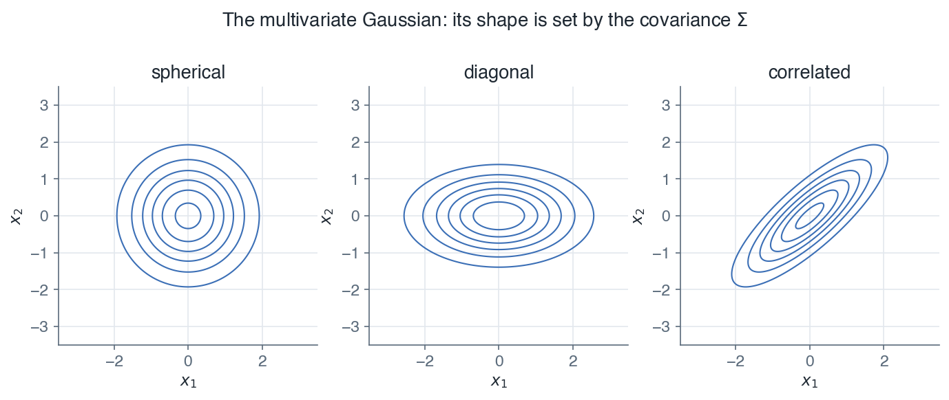+	*Une covariance sphérique donne des courbes circulaires, une covariance diagonale des ellipses alignées sur les axes, et les termes hors diagonale les inclinent, encodant la corrélation entre les caractéristiques.*
+
+	*Remarque :* la forme quadratique $(x - \mu)^T \Sigma^{-1}(x - \mu)$ est le carré de la distance de Mahalanobis, la distance naturelle une fois que les données ont une structure de covariance.
+
+	## 1.5 Vraisemblance, a priori, a posteriori et évidence
+
+	Presque tous les modèles de ce cours raisonnent sur des paramètres $\theta$ étant donné des données $D$. Quatre quantités reviennent, reliées entre elles par la règle de Bayes :
+
+	$$\boxed{ p(\theta \mid D) = \frac{p(D \mid \theta)\, p(\theta)}{p(D)} }$$
+
+	- La **vraisemblance** $p(D \mid \theta)$ est la probabilité des données pour un $\theta$ donné.
+	- L'**a priori** $p(\theta)$ est ce que l'on croyait sur $\theta$ avant de voir les données.
+	- L'**a posteriori** $p(\theta \mid D)$ est la croyance mise à jour après les avoir vues.
+	- L'**évidence** $p(D) = \int p(D \mid \theta)\, p(\theta)\, d\theta$ normalise l'a posteriori pour qu'il intègre à un.
+
+	
+
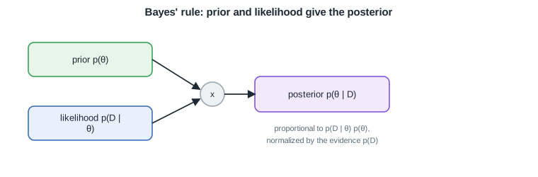+	*L'a posteriori est proportionnel à la vraisemblance fois l'a priori, divisé par l'évidence qui en fait une vraie distribution.*
+
+	*Remarque :* l'évidence est une constante par rapport à $\theta$, donc pour de nombreuses tâches on peut l'ignorer et seul le numérateur $p(D \mid \theta)\, p(\theta)$ compte.
+
+	*Ces outils sous-tendent le cours [Machine Learning](/fr/Machine%20Learning), où les probabilités, les fonctions de perte et les modèles s'appuient sur eux.*
+
+	---
+	Suivant : [Vue d'ensemble du cours](/fr/Mathematics)
/dev/null .. fr/Mathematics/01 Mathematical refresher/bayes-rule.svg
@@ 0,0 1,1 @@
+	<svg xmlns="http://www.w3.org/2000/svg" viewBox="0 0 760 250" width="760" height="250" font-family="Helvetica, Arial, sans-serif"><defs><marker id="arrow" viewBox="0 0 10 10" refX="8.5" refY="5" markerWidth="7" markerHeight="7" orient="auto-start-reverse"><path d="M0 0L10 5L0 10z" fill="#1f2933"/></marker><marker id="arrowmuted" viewBox="0 0 10 10" refX="8.5" refY="5" markerWidth="7" markerHeight="7" orient="auto-start-reverse"><path d="M0 0L10 5L0 10z" fill="#5b6b7b"/></marker></defs><rect width="760" height="250" fill="#ffffff"/><text x="380.0" y="22.0" font-family="Helvetica, Arial, sans-serif" font-size="15" font-weight="600" fill="#1f2933" text-anchor="middle">Bayes&#x27; rule: prior and likelihood give the posterior</text><rect x="40.0" y="60.0" width="175.0" height="48.0" rx="8" fill="#e7f5ea" stroke="#38a05a" stroke-width="1.6"/><text x="127.5" y="88.4" font-family="Helvetica, Arial, sans-serif" font-size="13" fill="#1f2933" text-anchor="middle">prior p(θ)</text><rect x="40.0" y="150.0" width="175.0" height="48.0" rx="8" fill="#e8f0fe" stroke="#3b6fb6" stroke-width="1.6"/><text x="127.5" y="170.8" font-family="Helvetica, Arial, sans-serif" font-size="13" fill="#1f2933" text-anchor="middle">likelihood p(D |</text><text x="127.5" y="186.1" font-family="Helvetica, Arial, sans-serif" font-size="13" fill="#1f2933" text-anchor="middle">θ)</text><circle cx="300.0" cy="133.0" r="17.0" fill="#eef1f4" stroke="#9aa7b2" stroke-width="1.6"/><text x="300.0" y="137.1" font-family="Helvetica, Arial, sans-serif" font-size="12" fill="#1f2933" text-anchor="middle">x</text><line x1="215.0" y1="84.0" x2="282.0" y2="126.0" stroke="#1f2933" stroke-width="1.7" marker-end="url(#arrow)"/><line x1="215.0" y1="174.0" x2="282.0" y2="140.0" stroke="#1f2933" stroke-width="1.7" marker-end="url(#arrow)"/><rect x="360.0" y="108.0" width="190.0" height="50.0" rx="8" fill="#f2e9fd" stroke="#8257d6" stroke-width="1.6"/><text x="455.0" y="137.4" font-family="Helvetica, Arial, sans-serif" font-size="13" fill="#1f2933" text-anchor="middle">posterior p(θ | D)</text><line x1="317.0" y1="133.0" x2="360.0" y2="133.0" stroke="#1f2933" stroke-width="1.7" marker-end="url(#arrow)"/><text x="455.0" y="185.0" font-family="Helvetica, Arial, sans-serif" font-size="11" fill="#5b6b7b" text-anchor="middle">proportional to p(D | θ) p(θ),</text><text x="455.0" y="202.0" font-family="Helvetica, Arial, sans-serif" font-size="11" fill="#5b6b7b" text-anchor="middle">normalized by the evidence p(D)</text></svg>
\	No newline at end of file
/dev/null .. fr/Mathematics/01 Mathematical refresher/multivariate-gaussian.png