
Blame
|
1 | # General concepts |
||||||
| 2 | ||||||||
| 3 | The building blocks shared by every supervised model: how a loss measures a single prediction and aggregates into a cost, how iterative optimization minimizes that cost, and how the probabilistic view (likelihood) recovers the same objectives. We close with Newton's method, a second-order alternative to gradient descent. |
|||||||
| 4 | ||||||||
| 5 | **Objectives** |
|||||||
| 6 | - Define a loss function and aggregate per-example losses into a single cost to minimize. |
|||||||
| 7 | - State the gradient descent update rule and contrast its batch and stochastic variants. |
|||||||
| 8 | - Define the likelihood and the MLE objective, and link it to minimizing a cost. |
|||||||
| 9 | - State Newton's update in one and several dimensions and compare it with gradient descent. |
|||||||
| 10 | ||||||||
| 11 | ## Loss functions and cost |
|||||||
| 12 | ||||||||
| 13 | ### Loss function |
|||||||
| 14 | ||||||||
| 15 | A loss function $L(z, y)$ is defined as a scalar penalty comparing a raw model score $z$ (or a predicted probability $\phi$) against the target $y$. Smaller is better. Each family of models is characterized by its loss. |
|||||||
| 16 | ||||||||
| 17 | | Loss | Formula $L(z,y)$ | Used by | |
|||||||
| 18 | | --- | --- | --- | |
|||||||
| 19 | | Least squared error | $\tfrac{1}{2}(y-z)^2$ | Linear regression | |
|||||||
| 20 | | Logistic | $\log\!\left(1+\exp(-yz)\right)$ | Logistic regression | |
|||||||
| 21 | | Hinge | $\max(0,\,1-yz)$ | SVM | |
|||||||
| 22 | | Cross-entropy | $-\left[\,y\log\phi+(1-y)\log(1-\phi)\,\right]$ | Neural networks | |
|||||||
| 23 | ||||||||
| 24 | *Remark:* $z$ denotes a raw score such as $\theta^T x$, whereas $\phi \in (0,1)$ denotes a predicted probability. The cross-entropy row takes a probability $\phi$, not a raw score. |
|||||||
| 25 | ||||||||
| 26 | ### Cost function |
|||||||
| 27 | ||||||||
| 28 | The cost $J(\theta)$ is defined as the sum of the per-example losses over the whole training set of $m$ examples: |
|||||||
| 29 | ||||||||
| 30 | $$\boxed{\,J(\theta)=\sum_{i=1}^{m} L\!\left(h_\theta(x^{(i)}),\,y^{(i)}\right)\,}$$ |
|||||||
| 31 | ||||||||
| 32 | Training a model means choosing $\theta$ to minimize $J(\theta)$. The next lesson shows how. |
|||||||
| 33 | ||||||||
| 34 | *Remark:* the factor $\tfrac{1}{2}$ in the squared error is a convention that cancels with the exponent when differentiating, leaving a clean gradient. |
|||||||
| 35 | ||||||||
| 36 | 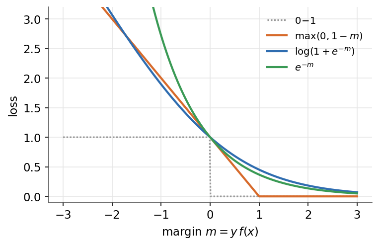 |
|||||||
| 37 | ||||||||
| 38 | *Margin-based losses, each a convex surrogate for the 0-1 loss that penalizes small or negative margins.* |
|||||||
| 39 | ||||||||
| 40 | ## Gradient descent |
|||||||
| 41 | ||||||||
| 42 | ### Update rule |
|||||||
| 43 | ||||||||
| 44 | Gradient descent iteratively moves the parameters $\theta$ against the gradient of the cost, scaled by a learning rate $\alpha > 0$: |
|||||||
| 45 | ||||||||
| 46 | $$\boxed{\,\theta \leftarrow \theta - \alpha\,\nabla_\theta J(\theta)\,}$$ |
|||||||
| 47 | ||||||||
| 48 | The gradient points in the direction of steepest increase, so stepping opposite to it decreases $J$. The step size $\alpha$ controls how far each update moves. |
|||||||
| 49 | ||||||||
| 50 | *Remark:* if $\alpha$ is too large the iterates can diverge, if too small convergence is slow. |
|||||||
| 51 | ||||||||
| 52 | ### Batch versus stochastic |
|||||||
| 53 | ||||||||
| 54 | The two variants differ in how many examples contribute to one update. |
|||||||
| 55 | ||||||||
| 56 | | Variant | Examples per update | Update | |
|||||||
| 57 | | --- | --- | --- | |
|||||||
| 58 | | Batch | All $m$ | $\theta \leftarrow \theta - \alpha\,\nabla_\theta J(\theta)$ | |
|||||||
| 59 | | Stochastic (SGD) | One $(x^{(i)}, y^{(i)})$ | $\theta \leftarrow \theta - \alpha\,\nabla_\theta L\!\left(h_\theta(x^{(i)}), y^{(i)}\right)$ | |
|||||||
| 60 | ||||||||
| 61 | Batch gives a smooth descent but reads the whole set per step. SGD updates after each example, so it is cheap per step and noisy. |
|||||||
| 62 | ||||||||
| 63 | ### LMS (Widrow-Hoff) update |
|||||||
| 64 | ||||||||
| 65 | For the least squared error, the per-coordinate stochastic update is defined as: |
|||||||
| 66 | ||||||||
| 67 | $$\boxed{\,\theta_j \leftarrow \theta_j + \alpha\left(y^{(i)} - h_\theta(x^{(i)})\right)x_j^{(i)}\,}$$ |
|||||||
| 68 | ||||||||
| 69 | The correction is proportional to the residual $y^{(i)} - h_\theta(x^{(i)})$ times the feature $x_j^{(i)}$. |
|||||||
| 70 | ||||||||
| 71 | *Remark:* a large residual produces a large step, a correct prediction produces no update. |
|||||||
| 72 | ||||||||
| 73 |  |
|||||||
| 74 | ||||||||
| 75 | *Gradient descent steps downhill toward the minimum (star).* |
|||||||
| 76 | ||||||||
| 77 | ## Likelihood and maximum likelihood estimation |
|||||||
| 78 | ||||||||
| 79 | ### Likelihood |
|||||||
| 80 | ||||||||
| 81 | The likelihood $L(\theta)$ is defined as the probability of the observed targets under the model, viewed as a function of the parameters $\theta$. Assuming examples are independent, it factorizes: |
|||||||
| 82 | ||||||||
| 83 | $$\boxed{\,L(\theta)=\prod_{i=1}^{m} p\!\left(y^{(i)} \mid x^{(i)}; \theta\right)\,}$$ |
|||||||
| 84 | ||||||||
| 85 | ### Log-likelihood |
|||||||
| 86 | ||||||||
| 87 | Products are awkward to optimize, so we take the logarithm. The log-likelihood $\ell(\theta)$ is defined as: |
|||||||
| 88 | ||||||||
| 89 | $$\boxed{\,\ell(\theta)=\sum_{i=1}^{m} \log p\!\left(y^{(i)} \mid x^{(i)}; \theta\right)\,}$$ |
|||||||
| 90 | ||||||||
| 91 | The $\log$ is monotone, so it has the same maximizer as $L(\theta)$ while turning the product into a sum. |
|||||||
| 92 | ||||||||
| 93 | ### Maximum likelihood estimation |
|||||||
| 94 | ||||||||
| 95 | The MLE is defined as the parameter value that makes the data most probable: |
|||||||
| 96 | ||||||||
| 97 | $$\boxed{\,\theta_{\mathrm{MLE}}=\arg\max_\theta\,\ell(\theta)\,}$$ |
|||||||
| 98 | ||||||||
| 99 | *Remark:* maximizing the log-likelihood is equivalent to minimizing the cost $J(\theta) = -\ell(\theta)$. This is exactly the cost-minimization view of the previous lessons, so likelihood and cost are two faces of one objective. |
|||||||
| 100 | ||||||||
| 101 | ## Newton's algorithm |
|||||||
| 102 | ||||||||
| 103 | ### One-dimensional update |
|||||||
| 104 | ||||||||
| 105 | To find a stationary point of the log-likelihood, Newton's method follows the local quadratic approximation. The scalar update is defined as: |
|||||||
| 106 | ||||||||
| 107 | $$\boxed{\,\theta \leftarrow \theta - \frac{\ell'(\theta)}{\ell''(\theta)}\,}$$ |
|||||||
| 108 | ||||||||
| 109 | It divides the first derivative by the second, so the step automatically adapts to the curvature. |
|||||||
| 110 | ||||||||
| 111 | ### Multivariate update |
|||||||
| 112 | ||||||||
| 113 | With a parameter vector $\theta \in \mathbb{R}^{n+1}$, the second derivative becomes the Hessian matrix $H$, with $H_{jk}=\dfrac{\partial^2 \ell}{\partial\theta_j\,\partial\theta_k}$. The update is defined as: |
|||||||
| 114 | ||||||||
| 115 | $$\boxed{\,\theta \leftarrow \theta - H^{-1}\,\nabla_\theta \ell(\theta)\,}$$ |
|||||||
| 116 | ||||||||
| 117 | *Remark:* each step solves a linear system in $H$, an $O(n^3)$ operation, so Newton's method is costly when the number of features $n$ is large. |
|||||||
| 118 | ||||||||
| 119 | ### Newton versus gradient descent |
|||||||
| 120 | ||||||||
| 121 | | Property | Newton's algorithm | Gradient descent | |
|||||||
| 122 | | --- | --- | --- | |
|||||||
| 123 | | Order | Second (uses curvature $H$) | First (uses gradient only) | |
|||||||
| 124 | | Per-step cost | High ($O(n^3)$, inverts $H$) | Low ($O(n)$ per example) | |
|||||||
| 125 | | Convergence | Quadratic near the optimum, few steps | Linear, many steps | |
|||||||
| 126 | | Tuning | No learning rate | Needs a learning rate $\alpha$ | |
|||||||
| 127 | ||||||||
| 128 | *Remark:* Newton's method converges in very few iterations but pays a high per-step cost, so gradient descent is preferred when $n$ is large. |
|||||||
| 129 | ||||||||
| 130 | *These tools are model-agnostic. The next part puts them to work on the simplest hypothesis class, where the prediction is a linear function of the features: linear models.* |
|||||||
| 131 | ||||||||
| 132 | --- |
|||||||
| 133 | Next: [Linear models](/en/Machine%20Learning/03%20Linear%20models) · [Course overview](/en/Machine%20Learning) |
|||||||