
General concepts
The building blocks shared by every supervised model: how a loss measures a single prediction and aggregates into a cost, how iterative optimization minimizes that cost, and how the probabilistic view (likelihood) recovers the same objectives. We close with Newton's method, a second-order alternative to gradient descent.
Objectives
- Define a loss function and aggregate per-example losses into a single cost to minimize.
- State the gradient descent update rule and contrast its batch and stochastic variants.
- Define the likelihood and the MLE objective, and link it to minimizing a cost.
- State Newton's update in one and several dimensions and compare it with gradient descent.
Loss functions and cost
Loss function
A loss function \(L(z, y)\) is defined as a scalar penalty comparing a raw model score \(z\) (or a predicted probability \(\phi\)) against the target \(y\). Smaller is better. Each family of models is characterized by its loss.
| Loss | Formula \(L(z,y)\) | Used by |
|---|---|---|
| Least squared error | \(\tfrac{1}{2}(y-z)^2\) | Linear regression |
| Logistic | \(\log\!\left(1+\exp(-yz)\right)\) | Logistic regression |
| Hinge | \(\max(0,\,1-yz)\) | SVM |
| Cross-entropy | \(-\left[\,y\log\phi+(1-y)\log(1-\phi)\,\right]\) | Neural networks |
Remark: \(z\) denotes a raw score such as \(\theta^T x\), whereas \(\phi \in (0,1)\) denotes a predicted probability. The cross-entropy row takes a probability \(\phi\), not a raw score.
Cost function
The cost \(J(\theta)\) is defined as the sum of the per-example losses over the whole training set of \(m\) examples:
\[\boxed{\,J(\theta)=\sum_{i=1}^{m} L\!\left(h_\theta(x^{(i)}),\,y^{(i)}\right)\,}\]Training a model means choosing \(\theta\) to minimize \(J(\theta)\). The next lesson shows how.
Remark: the factor \(\tfrac{1}{2}\) in the squared error is a convention that cancels with the exponent when differentiating, leaving a clean gradient.
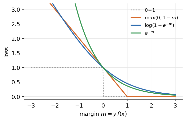
Margin-based losses, each a convex surrogate for the 0-1 loss that penalizes small or negative margins.
Gradient descent
Update rule
Gradient descent iteratively moves the parameters \(\theta\) against the gradient of the cost, scaled by a learning rate \(\alpha > 0\):
\[\boxed{\,\theta \leftarrow \theta - \alpha\,\nabla_\theta J(\theta)\,}\]The gradient points in the direction of steepest increase, so stepping opposite to it decreases \(J\). The step size \(\alpha\) controls how far each update moves.
Remark: if \(\alpha\) is too large the iterates can diverge, if too small convergence is slow.
Batch versus stochastic
The two variants differ in how many examples contribute to one update.
| Variant | Examples per update | Update |
|---|---|---|
| Batch | All \(m\) | \(\theta \leftarrow \theta - \alpha\,\nabla_\theta J(\theta)\) |
| Stochastic (SGD) | One \((x^{(i)}, y^{(i)})\) | \(\theta \leftarrow \theta - \alpha\,\nabla_\theta L\!\left(h_\theta(x^{(i)}), y^{(i)}\right)\) |
Batch gives a smooth descent but reads the whole set per step. SGD updates after each example, so it is cheap per step and noisy.
LMS (Widrow-Hoff) update
For the least squared error, the per-coordinate stochastic update is defined as:
\[\boxed{\,\theta_j \leftarrow \theta_j + \alpha\left(y^{(i)} - h_\theta(x^{(i)})\right)x_j^{(i)}\,}\]The correction is proportional to the residual \(y^{(i)} - h_\theta(x^{(i)})\) times the feature \(x_j^{(i)}\).
Remark: a large residual produces a large step, a correct prediction produces no update.

Gradient descent steps downhill toward the minimum (star).
Likelihood and maximum likelihood estimation
Likelihood
The likelihood \(L(\theta)\) is defined as the probability of the observed targets under the model, viewed as a function of the parameters \(\theta\). Assuming examples are independent, it factorizes:
\[\boxed{\,L(\theta)=\prod_{i=1}^{m} p\!\left(y^{(i)} \mid x^{(i)}; \theta\right)\,}\]Log-likelihood
Products are awkward to optimize, so we take the logarithm. The log-likelihood \(\ell(\theta)\) is defined as:
\[\boxed{\,\ell(\theta)=\sum_{i=1}^{m} \log p\!\left(y^{(i)} \mid x^{(i)}; \theta\right)\,}\]The \(\log\) is monotone, so it has the same maximizer as \(L(\theta)\) while turning the product into a sum.
Maximum likelihood estimation
The MLE is defined as the parameter value that makes the data most probable:
\[\boxed{\,\theta_{\mathrm{MLE}}=\arg\max_\theta\,\ell(\theta)\,}\]Remark: maximizing the log-likelihood is equivalent to minimizing the cost \(J(\theta) = -\ell(\theta)\). This is exactly the cost-minimization view of the previous lessons, so likelihood and cost are two faces of one objective.
Newton's algorithm
One-dimensional update
To find a stationary point of the log-likelihood, Newton's method follows the local quadratic approximation. The scalar update is defined as:
\[\boxed{\,\theta \leftarrow \theta - \frac{\ell'(\theta)}{\ell''(\theta)}\,}\]It divides the first derivative by the second, so the step automatically adapts to the curvature.
Multivariate update
With a parameter vector \(\theta \in \mathbb{R}^{n+1}\), the second derivative becomes the Hessian matrix \(H\), with \(H_{jk}=\dfrac{\partial^2 \ell}{\partial\theta_j\,\partial\theta_k}\). The update is defined as:
\[\boxed{\,\theta \leftarrow \theta - H^{-1}\,\nabla_\theta \ell(\theta)\,}\]Remark: each step solves a linear system in \(H\), an \(O(n^3)\) operation, so Newton's method is costly when the number of features \(n\) is large.
Newton versus gradient descent
| Property | Newton's algorithm | Gradient descent |
|---|---|---|
| Order | Second (uses curvature \(H\)) | First (uses gradient only) |
| Per-step cost | High (\(O(n^3)\), inverts \(H\)) | Low (\(O(n)\) per example) |
| Convergence | Quadratic near the optimum, few steps | Linear, many steps |
| Tuning | No learning rate | Needs a learning rate \(\alpha\) |
Remark: Newton's method converges in very few iterations but pays a high per-step cost, so gradient descent is preferred when \(n\) is large.
These tools are model-agnostic. The next part puts them to work on the simplest hypothesis class, where the prediction is a linear function of the features: linear models.
Next: Linear models · Course overview