Commit 1c3139

2026-06-30 12:04:21 Lucas Gonthier: Initial commit: course content (Machine Learning, MLOps) in EN and FR Co-Authored-By: Claude Opus 4.8 (1M context) <noreply@anthropic.com>

/dev/null .. .gitignore
@@ 0,0 1,3 @@
+	.DS_Store
+	*.swp
+	*~
/dev/null .. en.md
@@ 0,0 1,9 @@
+	# ML & MLOps Courses
+
+	Two courses on machine learning and putting it into production. Use the flags in the top bar to
+	change language.
+
+	## Courses
+
+	- [Machine Learning](/en/Machine%20Learning): foundations of ML, from data to models.
+	- [MLOps](/en/MLOps): taking ML systems to production and keeping them healthy.
/dev/null .. en/MLOps.md
@@ 0,0 1,19 @@
+	# MLOps
+
+	Taking machine learning systems to production: reproducibility, automation, deployment, and
+	monitoring.
+
+	**Prerequisites:** the [Machine Learning](/en/Machine%20Learning) course, basic command line and Git.
+
+	## Syllabus
+
+	1. [Introduction](/en/MLOps/01%20Introduction)
+	2. The ML Lifecycle *(planned)*
+	3. Experiment Tracking *(planned)*
+	4. Data and Model Versioning *(planned)*
+	5. Pipelines and Automation *(planned)*
+	6. Model Deployment *(planned)*
+	7. Monitoring and Observability *(planned)*
+
+	---
+	[Machine Learning](/en/Machine%20Learning) · [English home](/en)
/dev/null .. en/MLOps/01 Introduction.md
@@ 0,0 1,29 @@
+	# Introduction
+
+	> Lesson 01 · MLOps
+
+	**Objectives**
+	- Understand what MLOps is and why models need more than good accuracy.
+	- Recognize how ML systems differ from traditional software.
+	- See the lifecycle the rest of the course builds on.
+
+	## What is MLOps?
+
+	MLOps applies engineering and operations practices to the machine learning lifecycle so models
+	can be built, shipped, and maintained reliably and repeatably.
+
+	## Why it matters
+
+	A model that works in a notebook is not a product. Production adds data drift, reproducibility,
+	deployment, scaling, and monitoring concerns that the modelling step alone does not address.
+
+	## The ML lifecycle
+
+	1. Data collection and versioning.
+	2. Experimentation and tracking.
+	3. Training pipelines and automation.
+	4. Deployment.
+	5. Monitoring and feedback.
+
+	---
+	Next: The ML Lifecycle *(planned)* · [Course overview](/en/MLOps)
/dev/null .. en/Machine Learning.md
@@ 0,0 1,16 @@
+	# Machine Learning
+
+	Foundations of machine learning: how to go from raw data to a trained, evaluated model.
+
+	**Prerequisites:** basic Python, basic linear algebra and statistics.
+
+	## Syllabus
+
+	1. [Introduction](/en/Machine%20Learning/01%20Introduction)
+	2. [General concepts](/en/Machine%20Learning/02%20General%20concepts)
+	3. [Linear models](/en/Machine%20Learning/03%20Linear%20models)
+	4. [Support Vector Machines](/en/Machine%20Learning/04%20Support%20Vector%20Machines)
+	5. [Decision trees and ensemble methods](/en/Machine%20Learning/05%20Decision%20trees%20and%20ensemble%20methods)
+
+	---
+	[MLOps](/en/MLOps) · [English home](/en)
/dev/null .. en/Machine Learning/01 Introduction.md
@@ 0,0 1,115 @@
+	# Introduction
+
+	Machine learning builds models that learn patterns from data instead of being explicitly programmed with rules. This module fixes the notation used throughout the course and maps the landscape of problems and models, so later modules can stay terse and formula-first.
+
+	## Types of learning
+
+	- **Supervised**: learn from labelled examples (regression, classification).
+	- **Unsupervised**: find structure in unlabelled data (clustering, dimensionality reduction).
+	- **Reinforcement**: learn from feedback by interacting with an environment.
+
+	## The workflow
+
+	1. Define the problem and gather data.
+	2. Explore and preprocess the data.
+	3. Train candidate models.
+	4. Evaluate and compare them.
+	5. Deploy and monitor (see the [MLOps](/en/MLOps) course).
+
+	**Objectives**
+	- Fix the notation used across the whole course.
+	- Define the training set, the hypothesis, and the design matrix.
+	- Adopt the intercept convention $x_0 = 1$.
+	- Classify a supervised problem by the type of its output.
+	- Distinguish discriminative from generative models.
+
+	## Notation and setup
+
+	### Training set
+
+	The training set is defined as a collection of $m$ labelled examples:
+
+	$$\boxed{ \{(x^{(i)}, y^{(i)})\}_{i=1}^{m} }$$
+
+	Symbols:
+	- $x^{(i)}$ is the input (feature vector) of the $i$-th example.
+	- $y^{(i)}$ is its target (label).
+	- $m$ is the number of training examples.
+	- $n$ is the number of features.
+	- $x_j^{(i)}$ is the $j$-th feature of the $i$-th example.
+
+	*Remark:* the superscript $(i)$ indexes the example and the subscript $j$ indexes the feature, so $x_j^{(i)}$ is feature $j$ of example $i$.
+
+	By convention the input is augmented with a constant intercept term $x_0 = 1$, so $x \in \mathbb{R}^{n+1}$ and the parameters are $\theta \in \mathbb{R}^{n+1}$.
+
+	$$\boxed{ x_0 = 1, \quad x \in \mathbb{R}^{n+1}, \quad \theta \in \mathbb{R}^{n+1} }$$
+
+	*Remark:* the intercept lets a single dot product $\theta^T x$ carry the bias term, so no separate constant has to be written.
+
+	### Hypothesis
+
+	A hypothesis is defined as a function chosen from a model family that maps an input to a prediction:
+
+	$$\boxed{ h_\theta : x \mapsto h_\theta(x) }$$
+
+	Learning is the search, over the parameters $\theta$, for the hypothesis that best fits the training set.
+
+	### Design matrix
+
+	The design matrix stacks the $m$ transposed inputs row by row, and the target vector collects the labels:
+
+	$$\boxed{ X = \begin{bmatrix} (x^{(1)})^{T} \\ \vdots \\ (x^{(m)})^{T} \end{bmatrix}, \quad y = \begin{bmatrix} y^{(1)} \\ \vdots \\ y^{(m)} \end{bmatrix} }$$
+
+	Here $X \in \mathbb{R}^{m \times (n+1)}$ (each augmented input is a row) and $y \in \mathbb{R}^{m}$.
+
+	*Remark:* with this layout many models reduce to compact matrix expressions, for example a linear prediction over all examples is $X\theta$.
+
+	## Types of problems and models
+
+	### Type of prediction
+
+	A supervised problem is named by the nature of its target $y$.
+
+	| Type | Target | Goal |
+	| --- | --- | --- |
+	| Regression | $y \in \mathbb{R}$ | predict a continuous value |
+	| Classification | $y \in \{1, \dots, k\}$ | predict one of $k$ discrete classes |
+
+	*Remark:* binary classification is the case $k = 2$, often coded as $y \in \{0, 1\}$ or $y \in \{-1, +1\}$.
+
+	
+
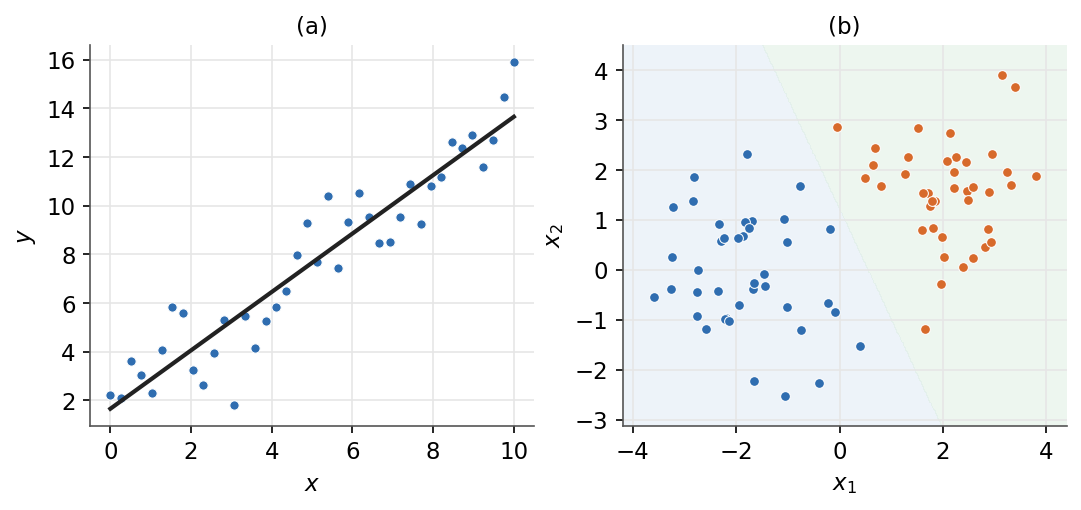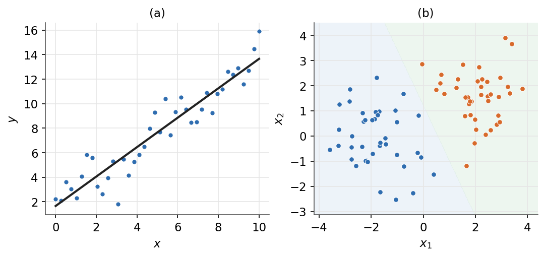
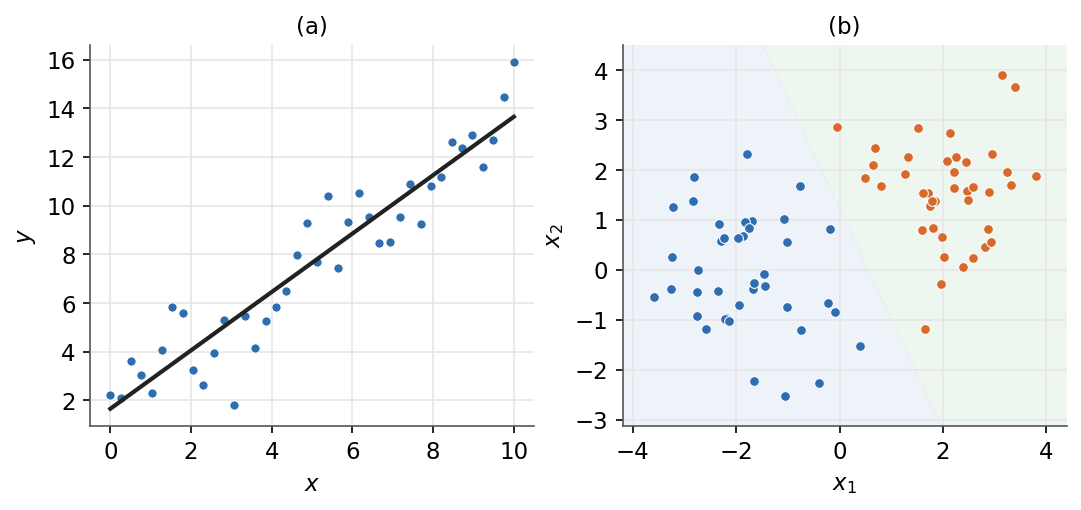
+	*Left: regression fits a continuous output. Right: classification separates the input space into classes.*
+
+	### Type of model
+
+	A model is discriminative if it learns the conditional $p(y \mid x)$ directly, and generative if it models how the data are generated, $p(x \mid y)$ and $p(y)$, then inverts via Bayes' rule:
+
+	$$\boxed{ p(y \mid x) = \frac{p(x \mid y)\, p(y)}{p(x)} }$$
+
+	| Aspect | Discriminative | Generative |
+	| --- | --- | --- |
+	| Goal | model the boundary between classes | model how each class generates data |
+	| What is learned | $p(y \mid x)$ directly | $p(x \mid y)$ and $p(y)$, then Bayes |
+	| Examples | logistic regression, SVM | Gaussian discriminant analysis, naive Bayes |
+
+	*Remark:* $p(x)$ is the same for every class, so for classification it can be dropped and the most probable class taken via $\arg\max_y\, p(x \mid y)\, p(y)$.
+
+	### Putting it together
+
+	The output type fixes regression vs classification, and the modelling choice fixes discriminative vs generative. Together they select a model family.
+
+	```mermaid
+	graph TD
+	A["supervised problem"] --> B{"output type?"}
+	B -->|"continuous"| C["regression"]
+	B -->|"discrete"| D["classification"]
+	D --> E{"model type?"}
+	E -->|"discriminative"| F["logistic regression, SVM"]
+	E -->|"generative"| G["GDA, naive Bayes"]
+	```
+
+	*With the problem framed and the notation fixed, the next part introduces the tools used to fit a model to data: loss functions, gradient descent, and maximum likelihood.*
+
+	---
+	Next: [General concepts](/en/Machine%20Learning/02%20General%20concepts) · [Course overview](/en/Machine%20Learning)
/dev/null .. en/Machine Learning/01 Introduction/regression-vs-classification.png
/dev/null .. en/Machine Learning/02 General concepts.md
@@ 0,0 1,133 @@
+	# General concepts
+
+	The building blocks shared by every supervised model: how a loss measures a single prediction and aggregates into a cost, how iterative optimization minimizes that cost, and how the probabilistic view (likelihood) recovers the same objectives. We close with Newton's method, a second-order alternative to gradient descent.
+
+	**Objectives**
+	- Define a loss function and aggregate per-example losses into a single cost to minimize.
+	- State the gradient descent update rule and contrast its batch and stochastic variants.
+	- Define the likelihood and the MLE objective, and link it to minimizing a cost.
+	- State Newton's update in one and several dimensions and compare it with gradient descent.
+
+	## Loss functions and cost
+
+	### Loss function
+
+	A loss function $L(z, y)$ is defined as a scalar penalty comparing a raw model score $z$ (or a predicted probability $\phi$) against the target $y$. Smaller is better. Each family of models is characterized by its loss.
+
+	| Loss | Formula $L(z,y)$ | Used by |
+	| --- | --- | --- |
+	| Least squared error | $\tfrac{1}{2}(y-z)^2$ | Linear regression |
+	| Logistic | $\log\!\left(1+\exp(-yz)\right)$ | Logistic regression |
+	| Hinge | $\max(0,\,1-yz)$ | SVM |
+	| Cross-entropy | $-\left[\,y\log\phi+(1-y)\log(1-\phi)\,\right]$ | Neural networks |
+
+	*Remark:* $z$ denotes a raw score such as $\theta^T x$, whereas $\phi \in (0,1)$ denotes a predicted probability. The cross-entropy row takes a probability $\phi$, not a raw score.
+
+	### Cost function
+
+	The cost $J(\theta)$ is defined as the sum of the per-example losses over the whole training set of $m$ examples:
+
+	$$\boxed{\,J(\theta)=\sum_{i=1}^{m} L\!\left(h_\theta(x^{(i)}),\,y^{(i)}\right)\,}$$
+
+	Training a model means choosing $\theta$ to minimize $J(\theta)$. The next lesson shows how.
+
+	*Remark:* the factor $\tfrac{1}{2}$ in the squared error is a convention that cancels with the exponent when differentiating, leaving a clean gradient.
+
+	
+
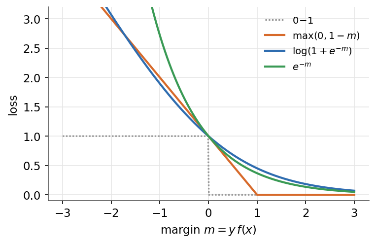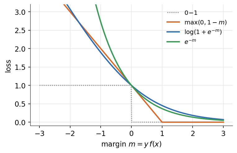
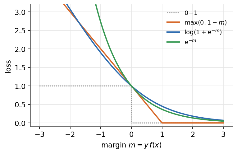
+	*Margin-based losses, each a convex surrogate for the 0-1 loss that penalizes small or negative margins.*
+
+	## Gradient descent
+
+	### Update rule
+
+	Gradient descent iteratively moves the parameters $\theta$ against the gradient of the cost, scaled by a learning rate $\alpha > 0$:
+
+	$$\boxed{\,\theta \leftarrow \theta - \alpha\,\nabla_\theta J(\theta)\,}$$
+
+	The gradient points in the direction of steepest increase, so stepping opposite to it decreases $J$. The step size $\alpha$ controls how far each update moves.
+
+	*Remark:* if $\alpha$ is too large the iterates can diverge, if too small convergence is slow.
+
+	### Batch versus stochastic
+
+	The two variants differ in how many examples contribute to one update.
+
+	| Variant | Examples per update | Update |
+	| --- | --- | --- |
+	| Batch | All $m$ | $\theta \leftarrow \theta - \alpha\,\nabla_\theta J(\theta)$ |
+	| Stochastic (SGD) | One $(x^{(i)}, y^{(i)})$ | $\theta \leftarrow \theta - \alpha\,\nabla_\theta L\!\left(h_\theta(x^{(i)}), y^{(i)}\right)$ |
+
+	Batch gives a smooth descent but reads the whole set per step. SGD updates after each example, so it is cheap per step and noisy.
+
+	### LMS (Widrow-Hoff) update
+
+	For the least squared error, the per-coordinate stochastic update is defined as:
+
+	$$\boxed{\,\theta_j \leftarrow \theta_j + \alpha\left(y^{(i)} - h_\theta(x^{(i)})\right)x_j^{(i)}\,}$$
+
+	The correction is proportional to the residual $y^{(i)} - h_\theta(x^{(i)})$ times the feature $x_j^{(i)}$.
+
+	*Remark:* a large residual produces a large step, a correct prediction produces no update.
+
+	
+
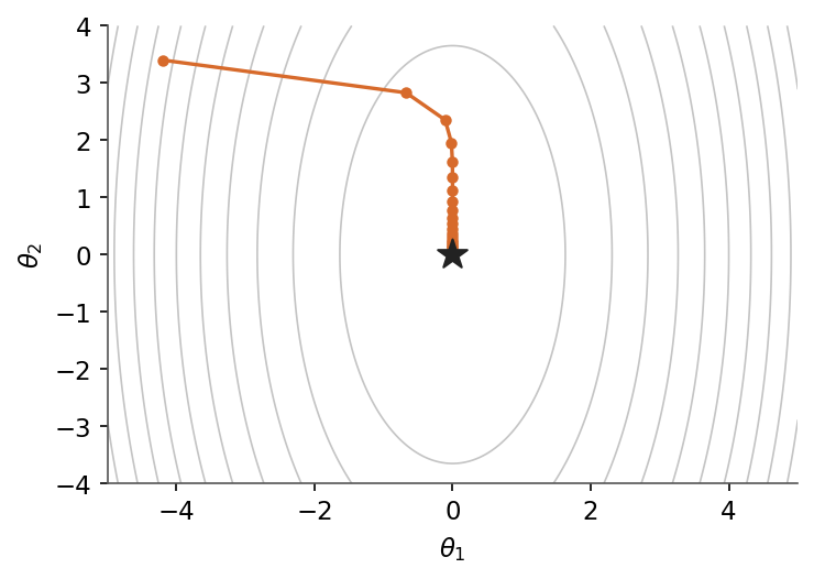
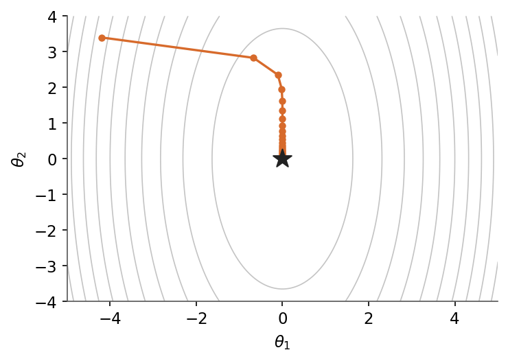
+	*Gradient descent steps downhill toward the minimum (star).*
+
+	## Likelihood and maximum likelihood estimation
+
+	### Likelihood
+
+	The likelihood $L(\theta)$ is defined as the probability of the observed targets under the model, viewed as a function of the parameters $\theta$. Assuming examples are independent, it factorizes:
+
+	$$\boxed{\,L(\theta)=\prod_{i=1}^{m} p\!\left(y^{(i)} \mid x^{(i)}; \theta\right)\,}$$
+
+	### Log-likelihood
+
+	Products are awkward to optimize, so we take the logarithm. The log-likelihood $\ell(\theta)$ is defined as:
+
+	$$\boxed{\,\ell(\theta)=\sum_{i=1}^{m} \log p\!\left(y^{(i)} \mid x^{(i)}; \theta\right)\,}$$
+
+	The $\log$ is monotone, so it has the same maximizer as $L(\theta)$ while turning the product into a sum.
+
+	### Maximum likelihood estimation
+
+	The MLE is defined as the parameter value that makes the data most probable:
+
+	$$\boxed{\,\theta_{\mathrm{MLE}}=\arg\max_\theta\,\ell(\theta)\,}$$
+
+	*Remark:* maximizing the log-likelihood is equivalent to minimizing the cost $J(\theta) = -\ell(\theta)$. This is exactly the cost-minimization view of the previous lessons, so likelihood and cost are two faces of one objective.
+
+	## Newton's algorithm
+
+	### One-dimensional update
+
+	To find a stationary point of the log-likelihood, Newton's method follows the local quadratic approximation. The scalar update is defined as:
+
+	$$\boxed{\,\theta \leftarrow \theta - \frac{\ell'(\theta)}{\ell''(\theta)}\,}$$
+
+	It divides the first derivative by the second, so the step automatically adapts to the curvature.
+
+	### Multivariate update
+
+	With a parameter vector $\theta \in \mathbb{R}^{n+1}$, the second derivative becomes the Hessian matrix $H$, with $H_{jk}=\dfrac{\partial^2 \ell}{\partial\theta_j\,\partial\theta_k}$. The update is defined as:
+
+	$$\boxed{\,\theta \leftarrow \theta - H^{-1}\,\nabla_\theta \ell(\theta)\,}$$
+
+	*Remark:* each step solves a linear system in $H$, an $O(n^3)$ operation, so Newton's method is costly when the number of features $n$ is large.
+
+	### Newton versus gradient descent
+
+	| Property | Newton's algorithm | Gradient descent |
+	| --- | --- | --- |
+	| Order | Second (uses curvature $H$) | First (uses gradient only) |
+	| Per-step cost | High ($O(n^3)$, inverts $H$) | Low ($O(n)$ per example) |
+	| Convergence | Quadratic near the optimum, few steps | Linear, many steps |
+	| Tuning | No learning rate | Needs a learning rate $\alpha$ |
+
+	*Remark:* Newton's method converges in very few iterations but pays a high per-step cost, so gradient descent is preferred when $n$ is large.
+
+	*These tools are model-agnostic. The next part puts them to work on the simplest hypothesis class, where the prediction is a linear function of the features: linear models.*
+
+	---
+	Next: [Linear models](/en/Machine%20Learning/03%20Linear%20models) · [Course overview](/en/Machine%20Learning)
/dev/null .. en/Machine Learning/02 General concepts/gradient-descent.png
/dev/null .. en/Machine Learning/02 General concepts/loss-functions.png
/dev/null .. en/Machine Learning/03 Linear models.md
@@ 0,0 1,193 @@
+	# Linear models
+
+	Linear models predict from a linear score $\theta^T x$. This module covers linear regression (continuous targets), logistic regression (binary classification), and the generalized linear model framework that unifies both through the exponential family. Each model is fit by maximum likelihood and shares the same gradient-based update.
+
+	**Objectives**
+	- Define the linear hypothesis and fit $\theta$ by the LMS update or the closed-form normal equation.
+	- See why least squares is the maximum-likelihood estimate under Gaussian noise.
+	- Map the linear score through the sigmoid and fit it by gradient ascent or Newton's method.
+	- Classify with the perceptron and know when its learning rule converges.
+	- Recognize the exponential-family form and build a GLM from its three assumptions.
+	- Recover linear, logistic, and softmax regression as special cases.
+
+	## Linear regression
+
+	### Hypothesis
+
+	The hypothesis is linear in the augmented input $x \in \mathbb{R}^{n+1}$ with $x_0 = 1$ and parameters $\theta \in \mathbb{R}^{n+1}$:
+
+	$$\boxed{ h_\theta(x) = \theta^T x }$$
+
+	### Cost function
+
+	The cost is defined as half the sum of squared residuals over the $m$ examples:
+
+	$$\boxed{ J(\theta) = \tfrac{1}{2}\sum_{i=1}^{m}\left(h_\theta(x^{(i)}) - y^{(i)}\right)^2 }$$
+
+	### LMS update
+
+	Gradient descent on $J$ gives the least-mean-squares (Widrow-Hoff) update, applied per example $(x^{(i)}, y^{(i)})$:
+
+	$$\boxed{ \theta_j \leftarrow \theta_j + \alpha\left(y^{(i)} - h_\theta(x^{(i)})\right)x_j^{(i)} }$$
+
+	with learning rate $\alpha > 0$.
+
+	| variant | update rule | per step | use when |
+	| --- | --- | --- | --- |
+	| Batch GD | sum over all $m$ examples | $O(mn)$ | $m$ small to moderate |
+	| Stochastic GD (SGD) | one example at a time | $O(n)$ | $m$ large, streaming |
+
+	### Normal equation
+
+	Setting $\nabla_\theta J(\theta) = 0$ gives a closed-form solution from the design matrix $X$ and target vector $y$:
+
+	$$\boxed{ \theta = (X^T X)^{-1}X^T y }$$
+
+	*Remark:* the normal equation needs no learning rate and no iteration, but inverting $X^T X$ costs $O(n^3)$, so for large $n$ the iterative LMS update is preferred.
+
+	### Probabilistic interpretation
+
+	Assume $y^{(i)} = \theta^T x^{(i)} + \varepsilon^{(i)}$ with i.i.d. Gaussian noise $\varepsilon^{(i)} \sim \mathcal{N}(0, \sigma^2)$. Maximizing the log-likelihood then coincides with minimizing the least-squares cost:
+
+	$$\boxed{ \arg\max_\theta \ell(\theta) = \arg\min_\theta J(\theta) }$$
+
+	*Remark:* this is why least squares is a principled objective and not merely a convenient one.
+
+	
+
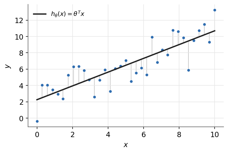
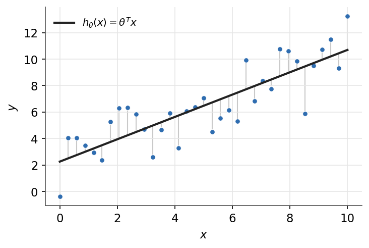
+	*Least squares fits the line that minimizes the squared residuals (grey segments).*
+
+	## Logistic regression
+
+	### Sigmoid
+
+	The sigmoid (logistic) function squashes a raw score $z \in \mathbb{R}$ into a probability:
+
+	$$\boxed{ g(z) = \frac{1}{1 + e^{-z}} \in (0, 1) }$$
+
+	Its derivative has the convenient form $g'(z) = g(z)\left(1 - g(z)\right)$.
+
+	### Model
+
+	The hypothesis outputs the probability of the positive class, with $\phi$ the predicted probability:
+
+	$$\boxed{ \phi = h_\theta(x) = g(\theta^T x) = p(y = 1 \mid x; \theta) }$$
+
+	Labels are $y \in \{0, 1\}$, so the conditional law is Bernoulli:
+
+	$$\boxed{ p(y \mid x; \theta) = \phi^{y}(1 - \phi)^{1 - y} }$$
+
+	### Log-likelihood
+
+	Over $m$ i.i.d. examples the log-likelihood is the negative cross-entropy summed over the data:
+
+	$$\boxed{ \ell(\theta) = \sum_{i=1}^{m}\left[ y^{(i)}\log \phi^{(i)} + (1 - y^{(i)})\log(1 - \phi^{(i)}) \right] }$$
+
+	with $\phi^{(i)} = h_\theta(x^{(i)})$.
+
+	### Gradient ascent
+
+	Maximizing $\ell$ by gradient ascent gives the same form as the LMS update:
+
+	$$\boxed{ \theta_j \leftarrow \theta_j + \alpha\left(y^{(i)} - h_\theta(x^{(i)})\right)x_j^{(i)} }$$
+
+	*Remark:* the update matches linear regression in form, even though $h_\theta$ is now the sigmoid. This is no coincidence, both are generalized linear models.
+
+	### Newton's method
+
+	Newton's method converges faster near the optimum. In one dimension:
+
+	$$\boxed{ \theta \leftarrow \theta - \frac{\ell'(\theta)}{\ell''(\theta)} }$$
+
+	In the vector case it uses the Hessian $H$ of $\ell$:
+
+	$$\boxed{ \theta \leftarrow \theta - H^{-1}\nabla_\theta \ell(\theta) }$$
+
+	*Remark:* logistic regression has no closed-form solution for $\theta$, so it is always fit iteratively (gradient ascent or Newton).
+
+	
+
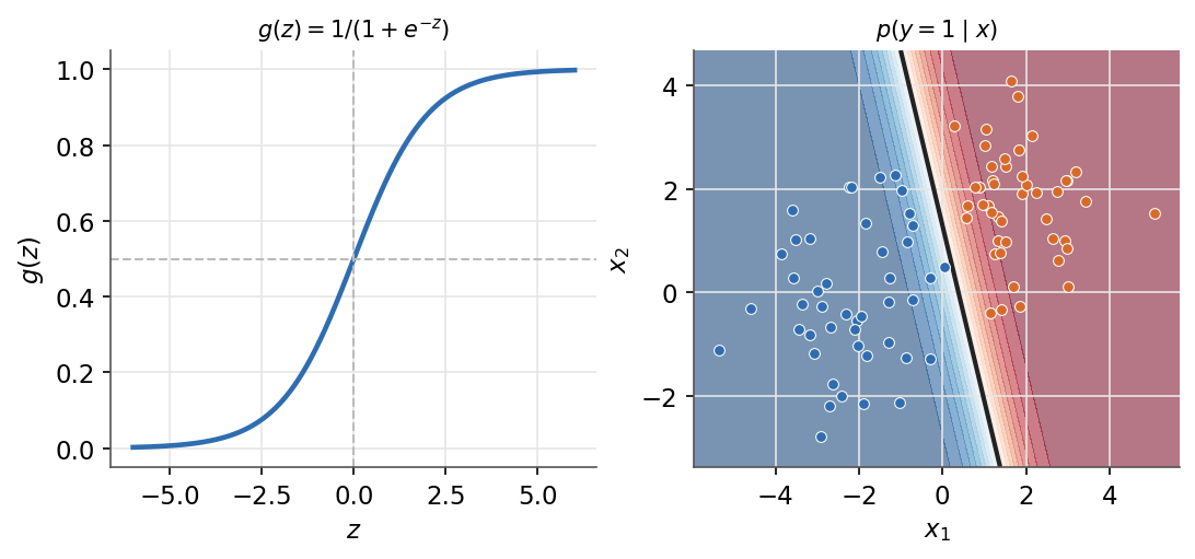
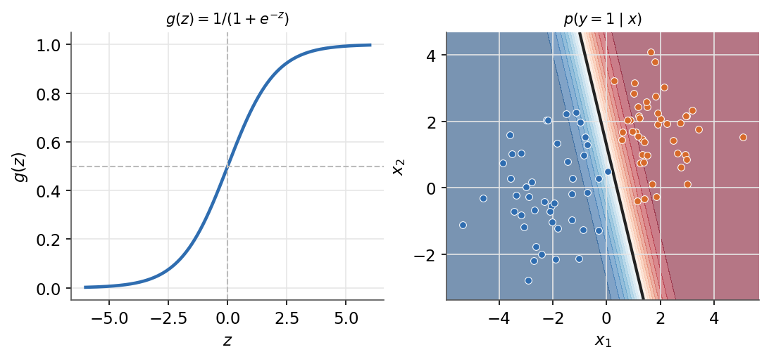
+	*Left: the sigmoid maps scores into the interval (0,1). Right: the decision boundary and predicted probability.*
+
+	## Perceptron
+
+	The perceptron is the original linear classifier. It keeps the linear score $\theta^T x$ of logistic regression but replaces the sigmoid with a hard threshold, so the output is a class label rather than a probability. Labels are $y \in \{0, 1\}$.
+
+	### Activation and hypothesis
+
+	The activation is the step function:
+
+	$$\boxed{ g(z) = \begin{cases} 1 & \text{if } z \ge 0 \\ 0 & \text{otherwise} \end{cases} }$$
+
+	and the hypothesis applies it to the linear score:
+
+	$$\boxed{ h_\theta(x) = g(\theta^T x) }$$
+
+	### Learning rule
+
+	The perceptron is trained online, one example at a time, and corrects $\theta$ only on a misclassified point:
+
+	$$\boxed{ \theta_j \leftarrow \theta_j + \alpha\left(y^{(i)} - h_\theta(x^{(i)})\right)x_j^{(i)} }$$
+
+	*Remark:* this is the same form as the LMS update and the logistic gradient-ascent update. Only the activation $g$ differs (identity, sigmoid, step). When the prediction is right the factor $y^{(i)} - h_\theta(x^{(i)})$ is zero, so correctly classified points leave $\theta$ unchanged.
+
+	
+
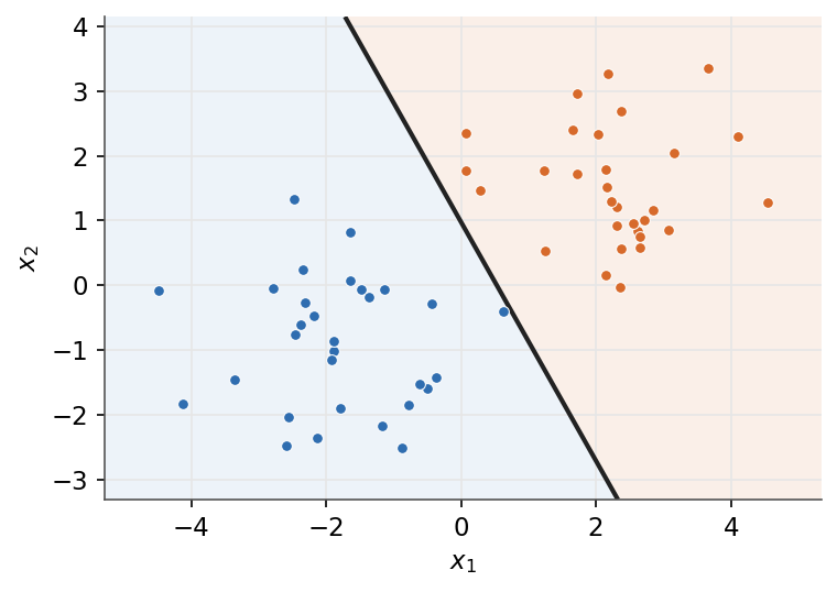
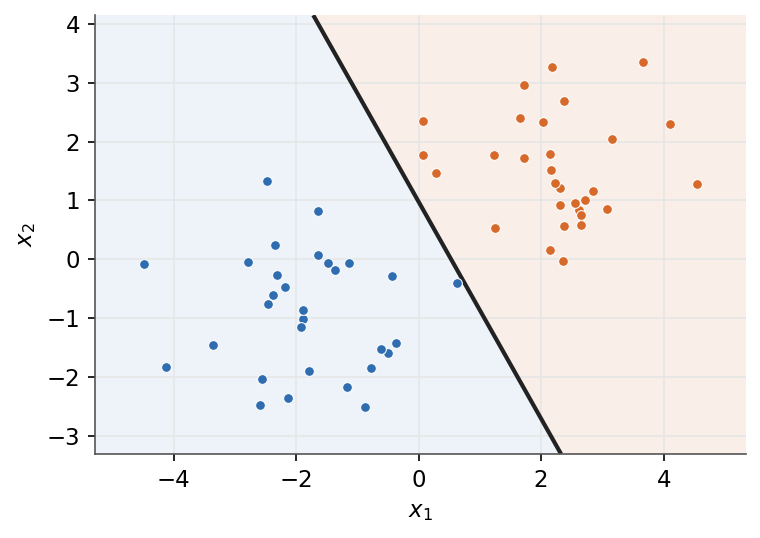
+	*The perceptron finds one separating hyperplane. It is not necessarily the maximum-margin one the SVM will choose.*
+
+	### Convergence
+
+	| data | behaviour |
+	| --- | --- |
+	| linearly separable | converges in a finite number of updates |
+	| not separable | never converges, the weights keep oscillating |
+
+	*Remark:* the perceptron stops at the first hyperplane that separates the data, usually not the one with the widest margin. This gap motivates the support vector machine (which maximizes the margin) and, stacked into layers, the neural network (a perceptron is a single unit).
+
+	## Generalized linear models
+
+	### Exponential family
+
+	A distribution is in the exponential family if its density can be written with natural parameter $\eta$, sufficient statistic $T(y)$, log-partition $a(\eta)$, and base measure $b(y)$:
+
+	$$\boxed{ p(y; \eta) = b(y)\exp\left(\eta\, T(y) - a(\eta)\right) }$$
+
+	### GLM assumptions
+
+	A GLM rests on three choices. The response is in the exponential family, the natural parameter is linear in the input, and the prediction is the expected sufficient statistic:
+
+	$$\boxed{ \eta = \theta^T x }$$
+
+	$$\boxed{ h_\theta(x) = \mathbb{E}\left[T(y) \mid x; \theta\right] }$$
+
+	### Family table
+
+	| Distribution | $\eta$ | $T(y)$ | $a(\eta)$ | $b(y)$ |
+	| --- | --- | --- | --- | --- |
+	| Bernoulli | $\log\dfrac{\phi}{1-\phi}$ | $y$ | $\log(1 + e^{\eta})$ | $1$ |
+	| Gaussian ($\sigma^2 = 1$) | $\mu$ | $y$ | $\tfrac{1}{2}\eta^2$ | $\dfrac{1}{\sqrt{2\pi}}e^{-y^2/2}$ |
+	| Poisson | $\log\lambda$ | $y$ | $e^{\eta}$ | $\dfrac{1}{y!}$ |
+	| Geometric | $\log(1-\phi)$ | $y$ | $\log\dfrac{e^{\eta}}{1 - e^{\eta}}$ | $1$ |
+
+	*Remark:* for the Bernoulli, $\eta$ is the log-odds and its inverse is the sigmoid, $\phi = g(\eta)$. This is why logistic regression has the form it does.
+
+	### Softmax regression
+
+	For multiclass labels $y \in \{1, \dots, k\}$ the GLM gives softmax regression, with one parameter vector $\theta_k$ per class:
+
+	$$\boxed{ p(y = k \mid x; \theta) = \frac{\exp(\theta_k^T x)}{\sum_{j}\exp(\theta_j^T x)} }$$
+
+	### GLM recipe
+
+	```mermaid
+	graph TD
+	A["pick a response distribution"] --> B["write it in exponential-family form"]
+	B --> C["set natural parameter eta linear in x"]
+	C --> D["prediction is expected sufficient statistic"]
+	D --> E["fit theta by maximum likelihood"]
+	```
+
+	*Linear models, including the perceptron, settle for any boundary that separates the classes. The next part asks for the best one: the support vector machine maximizes the margin.*
+
+	---
+	Next: [Support Vector Machines](/en/Machine%20Learning/04%20Support%20Vector%20Machines) · [Course overview](/en/Machine%20Learning)
/dev/null .. en/Machine Learning/03 Linear models/linear-regression.png
/dev/null .. en/Machine Learning/03 Linear models/logistic-regression.png
/dev/null .. en/Machine Learning/03 Linear models/perceptron.png
/dev/null .. en/Machine Learning/04 Support Vector Machines.md
@@ 0,0 1,215 @@
+	# Support Vector Machines
+
+	Support vector machines are large-margin linear classifiers. They pick the boundary that
+	maximizes the distance to the nearest points, control overfitting with the hinge loss and a
+	penalty $C$, and use kernels to fit nonlinear boundaries without ever forming the feature map.
+	Throughout, labels are $y \in \{-1,+1\}$ and the decision uses a raw score $z = w^T x - b$.
+
+	**Objectives**
+	- Define the SVM hypothesis, its separating hyperplane, and the geometric margin.
+	- State the hard-margin primal and the soft-margin primal with hinge loss and penalty $C$.
+	- Define kernels, the kernel trick, and the Mercer condition.
+	- Form the Lagrangian, derive the dual and KKT conditions, and define support vectors.
+
+	## Optimal margin classifier
+
+	Labels are $y \in \{-1,+1\}$, with weight vector $w \in \mathbb{R}^{n}$ and bias $b$.
+
+	### Hypothesis and boundary
+
+	The hypothesis is defined as the sign of the raw score $z = w^T x - b$:
+
+	$$\boxed{ h(x) = \operatorname{sign}(w^T x - b) }$$
+
+	The decision boundary is the set of points with zero score:
+
+	$$\boxed{ w^T x - b = 0 }$$
+
+	*Remark:* $w$ is orthogonal to the boundary, so it sets the orientation, and $b$ sets the offset.
+
+	### Geometric margin
+
+	The geometric margin of example $i$ is defined as its signed distance to the boundary, made
+	positive by the label:
+
+	$$\boxed{ \gamma^{(i)} = y^{(i)} \, \frac{w^T x^{(i)} - b}{\lVert w \rVert} }$$
+
+	A correctly classified point has $\gamma^{(i)} > 0$. The margin of the dataset is the smallest
+	$\gamma^{(i)}$ over all examples.
+
+	*Remark:* dividing by $\lVert w \rVert$ makes the margin invariant to rescaling $(w,b)$, unlike
+	the raw score $z$.
+
+	### Hard-margin primal
+
+	Fixing the scale so the closest points satisfy $y^{(i)}(w^T x^{(i)} - b) = 1$, maximizing the
+	margin is equivalent to minimizing $\lVert w \rVert^2$ subject to a unit functional margin:
+
+	$$\boxed{ \min_{w,b} \tfrac{1}{2}\lVert w \rVert^2 \quad \text{s.t.} \quad y^{(i)}(w^T x^{(i)} - b) \ge 1 \ \ \forall i }$$
+
+	This is a convex quadratic program with linear constraints, so it has a unique optimum.
+
+	*Remark:* it requires the data to be linearly separable. The next lesson relaxes that with slack
+	variables.
+
+	
+
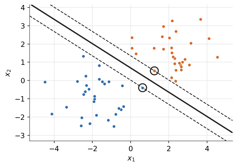
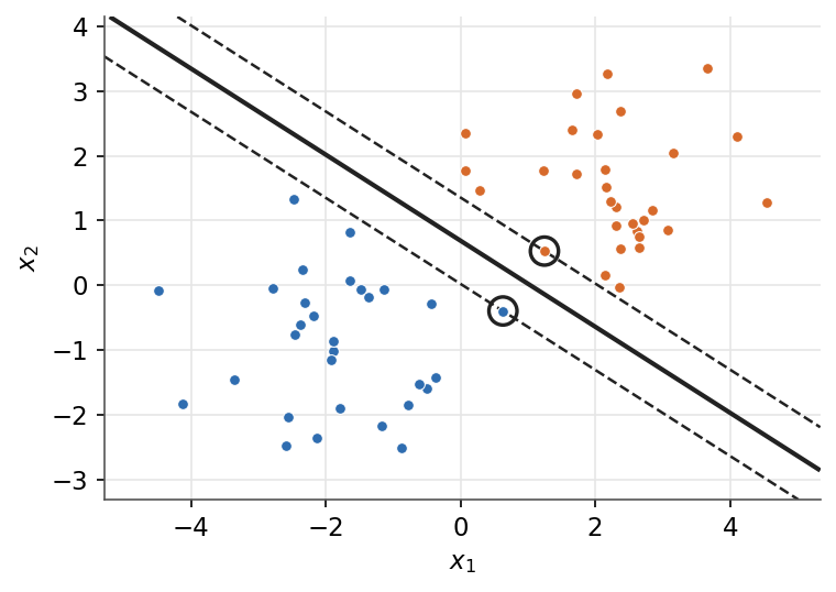
+	*The optimal hyperplane (solid) maximizes the margin (dashed). Circled points are the support vectors.*
+
+	## Hinge loss
+
+	The raw score is $z = w^T x - b$ and labels are $y \in \{-1,+1\}$.
+
+	### Hinge loss
+
+	The hinge loss is defined as the amount by which the margin $yz$ falls short of $1$, clipped at zero:
+
+	$$\boxed{ L(z,y) = \max(0,\, 1 - yz), \quad z = w^T x - b }$$
+
+	It is zero once $yz \ge 1$ (the point is correct and beyond the margin) and grows linearly inside
+	or past the margin.
+
+	*Remark:* the hinge loss is convex but not differentiable at $yz = 1$, so it is optimized with
+	subgradients.
+
+	### Soft-margin primal
+
+	Introduce a slack $\xi_i \ge 0$ per example to allow margin violations, penalized by $C > 0$:
+
+	$$\boxed{ \min_{w,b,\xi} \tfrac{1}{2}\lVert w \rVert^2 + C\sum_{i=1}^{m}\xi_i \quad \text{s.t.} \quad y^{(i)}(w^T x^{(i)} - b) \ge 1 - \xi_i, \ \ \xi_i \ge 0 }$$
+
+	At the optimum $\xi_i = \max(0,\, 1 - y^{(i)}(w^T x^{(i)} - b))$, so eliminating the slacks gives
+	the unconstrained regularized form:
+
+	$$\boxed{ \min_{w,b} \tfrac{1}{2}\lVert w \rVert^2 + C\sum_{i=1}^{m}\max\!\big(0,\, 1 - y^{(i)}(w^T x^{(i)} - b)\big) }$$
+
+	This is regularization plus hinge loss: the $\tfrac{1}{2}\lVert w \rVert^2$ term widens the margin
+	and the sum penalizes violations.
+
+	### Role of $C$
+
+	| $C$ | Penalty on violations | Margin | Behaviour |
+	| --- | --- | --- | --- |
+	| small | weak | wide | more violations tolerated, lower variance |
+	| large | strong | narrow | fewer violations, fits training data harder |
+
+	*Remark:* as $C \to \infty$ no violation is tolerated, which recovers the hard-margin classifier.
+
+	## Kernels
+
+	### Kernel definition
+
+	A kernel is defined as the inner product of a feature map $\phi$ applied to two inputs:
+
+	$$\boxed{ K(x,z) = \phi(x)^T \phi(z) }$$
+
+	A valid kernel computes this inner product directly, so $\phi$ never has to be formed (it may even
+	be infinite-dimensional).
+
+	### Kernel trick
+
+	The SVM dual depends on the data only through inner products $\langle x^{(i)}, x^{(j)} \rangle$.
+	The kernel trick replaces each inner product with a kernel:
+
+	$$\boxed{ \langle x^{(i)}, x^{(j)} \rangle \ \longrightarrow \ K(x^{(i)}, x^{(j)}) }$$
+
+	This fits a linear boundary in the feature space, which is nonlinear in the original space, at the
+	cost of evaluating $K$ instead of $\phi$.
+
+	A widely used choice is the Gaussian (RBF) kernel:
+
+	$$\boxed{ K(x,z) = \exp\!\left( -\frac{\lVert x - z \rVert^2}{2\sigma^2} \right) }$$
+
+	### Mercer condition
+
+	A function $K$ is a valid kernel if and only if, for every finite sample, its Gram matrix is
+	symmetric positive semidefinite:
+
+	$$\boxed{ K = K^T, \qquad K \succeq 0 }$$
+
+	*Remark:* this is the Mercer condition. It guarantees a feature map $\phi$ exists, so the dual stays
+	convex.
+
+	### Common kernels
+
+	| Kernel | $K(x,z)$ | Note |
+	| --- | --- | --- |
+	| Linear | $x^T z$ | no mapping, recovers the linear SVM |
+	| Polynomial | $(x^T z + c)^d$ | degree $d$, offset $c$ |
+	| Gaussian (RBF) | $\exp\!\big(-\tfrac{\lVert x - z \rVert^2}{2\sigma^2}\big)$ | infinite-dimensional, local |
+
+	*Remark:* a small $\sigma$ makes the RBF kernel very local, which can overfit. It trades off against
+	$C$.
+
+	
+
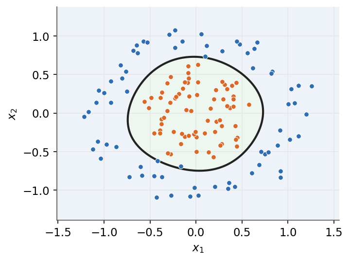
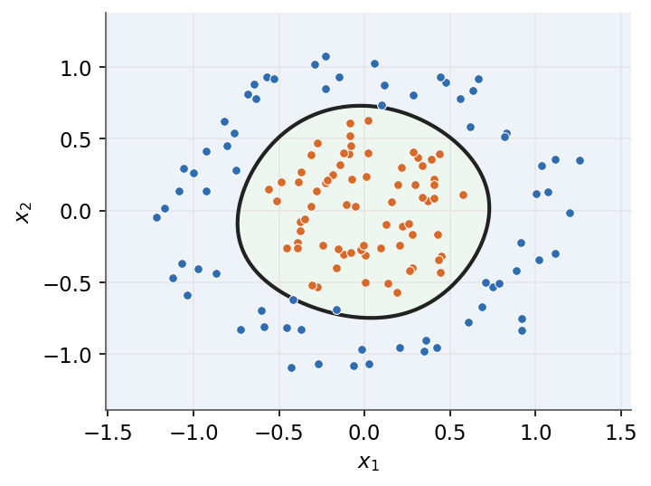
+	*An RBF kernel separates classes that are not linearly separable, with a nonlinear boundary in the input space.*
+
+	## Lagrangian and duality
+
+	### Lagrangian
+
+	For a primal objective $f(w)$ with inequality constraints $g_i(w) \le 0$ and multipliers
+	$\beta_i \ge 0$, the Lagrangian is defined as:
+
+	$$\boxed{ \mathcal{L}(w,\beta) = f(w) + \sum_{i=1}^{m} \beta_i \, g_i(w) }$$
+
+	Applied to the SVM primal $\tfrac{1}{2}\lVert w \rVert^2$ with constraints
+	$1 - y^{(i)}(w^T x^{(i)} - b) \le 0$, the stationarity conditions $\nabla_w \mathcal{L} = 0$ and
+	$\partial_b \mathcal{L} = 0$ give:
+
+	$$\boxed{ w = \sum_{i=1}^{m} \beta_i\, y^{(i)} x^{(i)}, \qquad \sum_{i=1}^{m} \beta_i\, y^{(i)} = 0 }$$
+
+	So the optimal $w$ is a linear combination of the training inputs weighted by $\beta_i y^{(i)}$.
+
+	### Dual problem
+
+	Substituting these back eliminates $w$ and $b$, leaving a problem in $\beta$ that depends on the
+	data only through inner products:
+
+	$$\boxed{ \max_{\beta} \ \sum_{i=1}^{m}\beta_i - \tfrac{1}{2}\sum_{i,j}\beta_i \beta_j\, y^{(i)} y^{(j)} \langle x^{(i)}, x^{(j)} \rangle \quad \text{s.t.} \quad \beta_i \ge 0, \ \ \sum_{i}\beta_i y^{(i)} = 0 }$$
+
+	The inner products are exactly where a kernel $K$ is substituted (see [Kernels](/en/Machine%20Learning/04%20Support%20Vector%20Machines#kernels)).
+
+	### KKT and support vectors
+
+	At the optimum, complementary slackness ties each multiplier to its constraint:
+
+	$$\boxed{ \beta_i \big[\, y^{(i)}(w^T x^{(i)} - b) - 1 \,\big] = 0 }$$
+
+	Support vectors are defined as the examples with a nonzero multiplier:
+
+	$$\boxed{ \text{support vectors} = \{\, i : \beta_i > 0 \,\} }$$
+
+	These are the points exactly on the margin. All others have $\beta_i = 0$ and do not affect $w$.
+
+	### Kernelized decision
+
+	Replacing the inner product by a kernel gives a decision rule expressed only through support vectors:
+
+	$$\boxed{ h(x) = \operatorname{sign}\!\left( \sum_{i=1}^{m} \beta_i\, y^{(i)}\, K(x^{(i)}, x) - b \right) }$$
+
+	*Remark:* only support vectors ($\beta_i > 0$) contribute, so prediction cost scales with their
+	count, not with $m$.
+
+	### From primal to decision
+
+	```mermaid
+	flowchart TD
+	A["primal QP: minimize half norm squared"]
+	B["Lagrangian with multipliers"]
+	C["dual problem in beta"]
+	D["KKT conditions"]
+	E["support vectors: beta greater than zero"]
+	F["kernelized decision rule"]
+	A --> B
+	B --> C
+	C --> D
+	D --> E
+	E --> F
+	```
+
+	*Support vector machines draw a single, possibly kernelized, boundary. The final part takes a different route: split the feature space with simple rules and combine many such models into an ensemble.*
+
+	---
+	Next: [Decision trees and ensemble methods](/en/Machine%20Learning/05%20Decision%20trees%20and%20ensemble%20methods) · [Course overview](/en/Machine%20Learning)
/dev/null .. en/Machine Learning/04 Support Vector Machines/svm-kernel.png
/dev/null .. en/Machine Learning/04 Support Vector Machines/svm-margin.png
/dev/null .. en/Machine Learning/05 Decision trees and ensemble methods.md
@@ 0,0 1,181 @@
+	# Decision trees and ensemble methods
+
+	Tree models partition the input space into axis-aligned regions and fit a constant per region, giving interpretable but high-variance predictors. Ensemble methods combine many trees: bagging and random forests average independently grown trees to cut variance, while boosting grows trees sequentially to cut bias.
+
+	**Objectives**
+	- Express a tree as a piecewise-constant function and choose splits with an impurity criterion.
+	- Control overfitting with cost-complexity pruning.
+	- Reduce variance by bagging and decorrelate trees with feature subsampling.
+	- Estimate generalization error for free with out-of-bag samples.
+	- Build a strong predictor as an additive sum of weak learners (AdaBoost, gradient boosting).
+
+	## CART decision trees
+
+	### Tree as a partition
+
+	A CART tree partitions the input space into $M$ disjoint regions $R_1,\dots,R_M$ (the leaves) and predicts a constant $c_m$ on each. The prediction is defined as
+
+	$$\boxed{ h(x)=\sum_{m=1}^{M} c_m\,\mathbf{1}\{x\in R_m\} }$$
+
+	Each internal node tests one feature against a threshold, $x_j\le s$, sending an example left or right. A path from the root to a leaf is a conjunction of such tests.
+
+	*Remark:* the regions are axis-aligned boxes, so the decision boundary is a staircase. A single tree has low bias but high variance.
+
+	### Impurity and split selection
+
+	For a region with class proportions $\hat p_k$, impurity measures how mixed the labels are. The Gini index is defined as
+
+	$$\boxed{ G = 1-\sum_{k}\hat p_k^{\,2} }$$
+
+	and the entropy as
+
+	$$\boxed{ H = -\sum_{k}\hat p_k\log_2\hat p_k }$$
+
+	A candidate split sends $N_-$ examples to child $R_-$ and $N_+$ to child $R_+$ out of $N$. Its information gain is defined as
+
+	$$\boxed{ IG = I(\text{parent})-\frac{N_-}{N}\,I(R_-)-\frac{N_+}{N}\,I(R_+) }$$
+
+	where $I$ is the chosen impurity. CART greedily picks the feature and threshold that maximize $IG$ at each node.
+
+	| criterion | formula | range (binary) | note |
+	| --- | --- | --- | --- |
+	| Gini | $1-\sum_k\hat p_k^{2}$ | $[0,0.5]$ | cheaper, no logarithm |
+	| entropy | $-\sum_k\hat p_k\log_2\hat p_k$ | $[0,1]$ | information-theoretic |
+
+	*Remark:* the two criteria almost always pick the same split. Gini is the default in most implementations because it avoids the logarithm.
+
+	### Regression trees
+
+	For regression the leaf value is the mean of the targets in the region, defined as
+
+	$$\boxed{ c_m=\frac{1}{N_m}\sum_{x^{(i)}\in R_m} y^{(i)} }$$
+
+	and splits minimize the within-region squared error instead of a classification impurity.
+
+	### Pruning
+
+	An unpruned tree fits the training set exactly and overfits. Cost-complexity pruning trades fit against tree size $|T|$ (the number of leaves) through a penalty $\alpha\ge0$:
+
+	$$\boxed{ C_\alpha(T)=\sum_{m} N_m\,I(R_m)+\alpha\,|T| }$$
+
+	Increasing $\alpha$ collapses the weakest splits, yielding a nested sequence of subtrees. The best $\alpha$ is chosen by cross-validation.
+
+	```mermaid
+	graph TD
+	A["x_j <= s ?"] -->|"yes"| B["x_k <= t ?"]
+	A -->|"no"| C["leaf R3"]
+	B -->|"yes"| D["leaf R1"]
+	B -->|"no"| E["leaf R2"]
+	```
+
+	
+
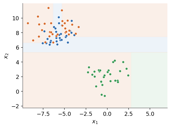
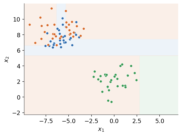
+	*A tree carves the input space into axis-aligned regions, each with a constant prediction.*
+
+	## Random forests
+
+	### Bagging
+
+	Bagging (bootstrap aggregating) trains $B$ trees on $B$ bootstrap resamples of the data and averages them. The bagged predictor is defined as
+
+	$$\boxed{ h_{\text{bag}}(x)=\frac{1}{B}\sum_{b=1}^{B} h_b(x) }$$
+
+	For classification the average is replaced by a majority vote. Averaging leaves bias unchanged while shrinking variance.
+
+	A bootstrap sample draws $N$ examples with replacement from $N$ examples. The probability that a given example is never drawn is $(1-\tfrac1N)^N\to e^{-1}\approx0.37$, so about 37% of the data is left out of each tree. These are its out-of-bag (OOB) examples.
+
+	### Variance of an average
+
+	If the $B$ trees each have variance $\sigma^2$ and pairwise correlation $\rho$, the variance of their average is
+
+	$$\boxed{ \rho\sigma^2+\frac{1-\rho}{B}\,\sigma^2 }$$
+
+	The second term vanishes as $B$ grows, but the first, $\rho\sigma^2$, does not. Reducing the correlation $\rho$ between trees is therefore the key lever, and that is what random forests target.
+
+	### Random forests
+
+	A random forest is bagging plus feature subsampling: at each split only a random subset of $m_{\text{try}}$ features is considered as split candidates. The usual choices are
+
+	$$\boxed{ m_{\text{try}}=\lfloor\sqrt{n}\,\rfloor\ \text{(classification)},\qquad m_{\text{try}}=\lfloor n/3\rfloor\ \text{(regression)} }$$
+
+	Restricting the candidate features stops every tree from splitting on the same dominant feature, which decorrelates the trees and lowers $\rho$.
+
+	*Remark:* OOB error averages each tree's error over only the examples that tree never saw, giving a cross-validation-like estimate at no extra cost.
+
+	| property | bagging | random forest |
+	| --- | --- | --- |
+	| resampling | bootstrap | bootstrap |
+	| split candidates | all $n$ features | random $m_{\text{try}}$ features |
+	| tree correlation $\rho$ | higher | lower |
+	| variance reduction | moderate | stronger |
+
+	```mermaid
+	graph TD
+	A["training set"] --> B1["bootstrap sample 1"]
+	A --> B2["bootstrap sample 2"]
+	A --> B3["bootstrap sample B"]
+	B1 --> T1["tree 1"]
+	B2 --> T2["tree 2"]
+	B3 --> T3["tree B"]
+	T1 --> AGG["aggregate: average or vote"]
+	T2 --> AGG
+	T3 --> AGG
+	```
+
+	
+
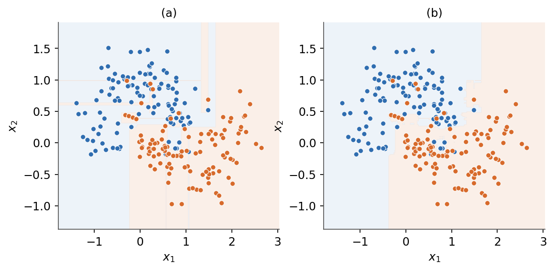
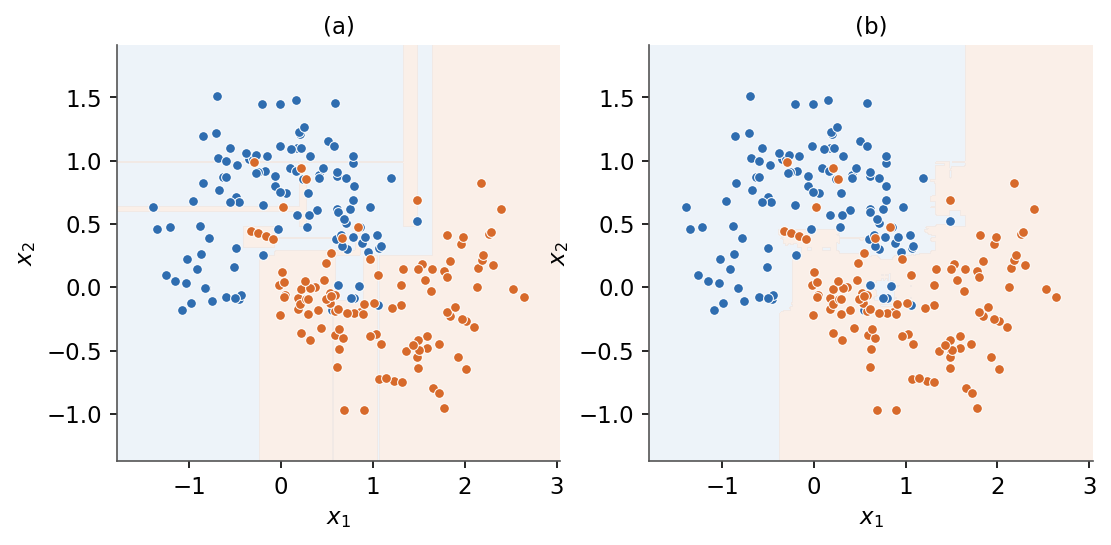
+	*(a) A single deep tree overfits with a jagged boundary. (b) A random forest averages many trees for a smoother boundary.*
+
+	## Boosting
+
+	### Additive model
+
+	Boosting builds a predictor as a weighted sum of $T$ weak learners $h_t$ (typically shallow trees), fitted one at a time. The additive model is defined as
+
+	$$\boxed{ H_T(x)=\sum_{t=1}^{T}\alpha_t\,h_t(x) }$$
+
+	Each stage corrects the errors of the running sum, so the ensemble is built sequentially and reduces bias rather than variance.
+
+	### AdaBoost
+
+	With labels $y\in\{-1,+1\}$, AdaBoost keeps example weights $w^{(i)}$ that concentrate on the currently misclassified points. At round $t$ the weak learner has weighted error $\varepsilon_t$, and its coefficient is defined as
+
+	$$\boxed{ \alpha_t=\tfrac12\log\frac{1-\varepsilon_t}{\varepsilon_t} }$$
+
+	so a more accurate learner ($\varepsilon_t$ small) gets a larger vote. The weights are then updated as
+
+	$$\boxed{ w^{(i)}\leftarrow w^{(i)}\exp\!\big(-\alpha_t\,y^{(i)}h_t(x^{(i)})\big) }$$
+
+	and renormalized. Misclassified examples ($y^{(i)}h_t(x^{(i)})<0$) gain weight, so the next learner focuses on them.
+
+	### Gradient boosting
+
+	Gradient boosting generalizes the idea to any differentiable loss $L$. At stage $t$ it fits the next learner to the negative gradient of the loss evaluated at the current model, the pseudo-residual defined as
+
+	$$\boxed{ r^{(i)}_t=-\left[\frac{\partial L\big(y^{(i)},f(x^{(i)})\big)}{\partial f}\right]_{f=H_{t-1}} }$$
+
+	The model is then updated with a learning rate (shrinkage) $\nu\in(0,1]$:
+
+	$$\boxed{ H_t=H_{t-1}+\nu\,\alpha_t\,h_t }$$
+
+	*Remark:* with squared-error loss the pseudo-residual is just the ordinary residual $y^{(i)}-H_{t-1}(x^{(i)})$, so each tree fits what the current model still gets wrong.
+
+	| property | bagging | boosting |
+	| --- | --- | --- |
+	| training | parallel, independent | sequential, each on the previous errors |
+	| base learners | deep, low bias | shallow, high bias |
+	| mainly reduces | variance | bias |
+	| reweighting | none (bootstrap) | weights or pseudo-residuals |
+
+	```mermaid
+	graph LR
+	A["weak learner 1"] --> B["weak learner 2"]
+	B --> C["weak learner 3"]
+	C --> D["weak learner T"]
+	D --> E["weighted sum H_T"]
+	```
+
+	*This completes the supervised-learning core of the course. To take these models from a notebook to a running service, continue with the [MLOps](/en/MLOps) course.*
+
+	---
+	Next: [Course overview](/en/Machine%20Learning)
/dev/null .. en/Machine Learning/05 Decision trees and ensemble methods/forest-vs-tree.png
/dev/null .. en/Machine Learning/05 Decision trees and ensemble methods/tree-boundary.png
/dev/null .. fr.md
@@ 0,0 1,9 @@
+	# Cours ML & MLOps
+
+	Deux cours sur le machine learning et sa mise en production. Utilisez les drapeaux en haut de la
+	page pour changer de langue.
+
+	## Cours
+
+	- [Machine Learning](/fr/Machine%20Learning) : les fondements du ML, des données aux modèles.
+	- [MLOps](/fr/MLOps) : mettre les systèmes de ML en production et les maintenir.
/dev/null .. fr/MLOps.md
@@ 0,0 1,19 @@
+	# MLOps
+
+	Mettre les systèmes de machine learning en production : reproductibilité, automatisation,
+	déploiement et surveillance.
+
+	**Prérequis :** le cours [Machine Learning](/fr/Machine%20Learning), bases de la ligne de commande et de Git.
+
+	## Programme
+
+	1. [Introduction](/fr/MLOps/01%20Introduction)
+	2. Le cycle de vie du ML *(à venir)*
+	3. Suivi des expériences *(à venir)*
+	4. Versionnage des données et des modèles *(à venir)*
+	5. Pipelines et automatisation *(à venir)*
+	6. Déploiement des modèles *(à venir)*
+	7. Surveillance et observabilité *(à venir)*
+
+	---
+	[Machine Learning](/fr/Machine%20Learning) · [Accueil français](/fr)
/dev/null .. fr/MLOps/01 Introduction.md
@@ 0,0 1,30 @@
+	# Introduction
+
+	> Leçon 01 · MLOps
+
+	**Objectifs**
+	- Comprendre ce qu'est le MLOps et pourquoi un bon score ne suffit pas.
+	- Voir en quoi les systèmes de ML diffèrent du logiciel classique.
+	- Découvrir le cycle de vie sur lequel s'appuie le reste du cours.
+
+	## Qu'est-ce que le MLOps ?
+
+	Le MLOps applique les pratiques d'ingénierie et d'exploitation au cycle de vie du machine
+	learning, afin de construire, livrer et maintenir des modèles de façon fiable et reproductible.
+
+	## Pourquoi c'est important
+
+	Un modèle qui fonctionne dans un notebook n'est pas un produit. La production ajoute la dérive
+	des données, la reproductibilité, le déploiement, la mise à l'échelle et la surveillance, que
+	l'étape de modélisation seule ne couvre pas.
+
+	## Le cycle de vie du ML
+
+	1. Collecte et versionnage des données.
+	2. Expérimentation et suivi.
+	3. Pipelines d'entraînement et automatisation.
+	4. Déploiement.
+	5. Surveillance et retours.
+
+	---
+	Suivant : Le cycle de vie du ML *(à venir)* · [Vue d'ensemble du cours](/fr/MLOps)
/dev/null .. fr/Machine Learning.md
@@ 0,0 1,16 @@
+	# Machine Learning
+
+	Les fondements du machine learning : passer de données brutes à un modèle entraîné et évalué.
+
+	**Prérequis :** Python de base, notions d'algèbre linéaire et de statistiques.
+
+	## Programme
+
+	1. [Introduction](/fr/Machine%20Learning/01%20Introduction)
+	2. [Concepts généraux](/fr/Machine%20Learning/02%20General%20concepts)
+	3. [Modèles linéaires](/fr/Machine%20Learning/03%20Linear%20models)
+	4. [Machines à vecteurs de support](/fr/Machine%20Learning/04%20Support%20Vector%20Machines)
+	5. [Arbres de décision et méthodes d'ensemble](/fr/Machine%20Learning/05%20Decision%20trees%20and%20ensemble%20methods)
+
+	---
+	[MLOps](/fr/MLOps) · [Accueil français](/fr)
/dev/null .. fr/Machine Learning/01 Introduction.md
@@ 0,0 1,115 @@
+	# Introduction
+
+	Le machine learning construit des modèles qui apprennent des motifs à partir de données, au lieu d'être programmés explicitement avec des règles. Ce module fixe la notation utilisée tout au long du cours et cartographie l'éventail des problèmes et des modèles, afin que les modules suivants restent concis et centrés sur les formules.
+
+	## Types d'apprentissage
+
+	- **Supervisé** : apprendre à partir d'exemples étiquetés (régression, classification).
+	- **Non supervisé** : trouver une structure dans des données non étiquetées (clustering, réduction de dimension).
+	- **Par renforcement** : apprendre via des retours en interagissant avec un environnement.
+
+	## Le déroulé
+
+	1. Définir le problème et rassembler les données.
+	2. Explorer et préparer les données.
+	3. Entraîner des modèles candidats.
+	4. Les évaluer et les comparer.
+	5. Déployer et surveiller (voir le cours [MLOps](/fr/MLOps)).
+
+	**Objectifs**
+	- Fixer la notation utilisée dans tout le cours.
+	- Définir l'ensemble d'entraînement, l'hypothèse et la matrice de conception.
+	- Adopter la convention d'ordonnée à l'origine $x_0 = 1$.
+	- Classer un problème supervisé selon le type de sa sortie.
+	- Distinguer les modèles discriminatifs des modèles génératifs.
+
+	## Notation et mise en place
+
+	### Ensemble d'entraînement
+
+	L'ensemble d'entraînement est défini comme une collection de $m$ exemples étiquetés :
+
+	$$\boxed{ \{(x^{(i)}, y^{(i)})\}_{i=1}^{m} }$$
+
+	Symboles :
+	- $x^{(i)}$ est l'entrée (vecteur de caractéristiques) du $i$-ème exemple.
+	- $y^{(i)}$ est sa cible (étiquette).
+	- $m$ est le nombre d'exemples d'entraînement.
+	- $n$ est le nombre de caractéristiques.
+	- $x_j^{(i)}$ est la $j$-ème caractéristique du $i$-ème exemple.
+
+	*Remarque :* l'exposant $(i)$ indexe l'exemple et l'indice $j$ indexe la caractéristique, donc $x_j^{(i)}$ est la caractéristique $j$ de l'exemple $i$.
+
+	Par convention l'entrée est augmentée d'un terme d'ordonnée à l'origine constant $x_0 = 1$, donc $x \in \mathbb{R}^{n+1}$ et les paramètres sont $\theta \in \mathbb{R}^{n+1}$.
+
+	$$\boxed{ x_0 = 1, \quad x \in \mathbb{R}^{n+1}, \quad \theta \in \mathbb{R}^{n+1} }$$
+
+	*Remarque :* l'ordonnée à l'origine permet à un seul produit scalaire $\theta^T x$ de porter le terme de biais, de sorte qu'aucune constante séparée n'a besoin d'être écrite.
+
+	### Hypothèse
+
+	Une hypothèse est définie comme une fonction choisie dans une famille de modèles qui associe une entrée à une prédiction :
+
+	$$\boxed{ h_\theta : x \mapsto h_\theta(x) }$$
+
+	L'apprentissage est la recherche, sur les paramètres $\theta$, de l'hypothèse qui s'ajuste le mieux à l'ensemble d'entraînement.
+
+	### Matrice de conception
+
+	La matrice de conception empile les $m$ entrées transposées ligne par ligne, et le vecteur cible rassemble les étiquettes :
+
+	$$\boxed{ X = \begin{bmatrix} (x^{(1)})^{T} \\ \vdots \\ (x^{(m)})^{T} \end{bmatrix}, \quad y = \begin{bmatrix} y^{(1)} \\ \vdots \\ y^{(m)} \end{bmatrix} }$$
+
+	Ici $X \in \mathbb{R}^{m \times (n+1)}$ (chaque entrée augmentée est une ligne) et $y \in \mathbb{R}^{m}$.
+
+	*Remarque :* avec cette disposition de nombreux modèles se réduisent à des expressions matricielles compactes, par exemple une prédiction linéaire sur tous les exemples vaut $X\theta$.
+
+	## Types de problèmes et de modèles
+
+	### Type de prédiction
+
+	Un problème supervisé est nommé selon la nature de sa cible $y$.
+
+	| Type | Cible | Objectif |
+	| --- | --- | --- |
+	| Régression | $y \in \mathbb{R}$ | prédire une valeur continue |
+	| Classification | $y \in \{1, \dots, k\}$ | prédire l'une des $k$ classes discrètes |
+
+	*Remarque :* la classification binaire est le cas $k = 2$, souvent codé $y \in \{0, 1\}$ ou $y \in \{-1, +1\}$.
+
+	
+
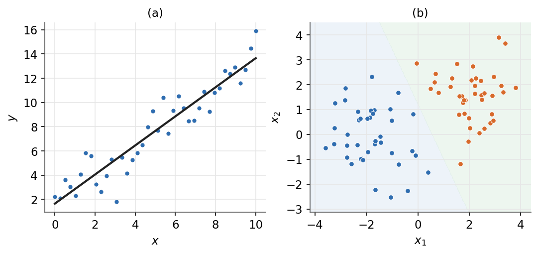+	*À gauche : la régression ajuste une sortie continue. À droite : la classification sépare l'espace en classes.*
+
+	### Type de modèle
+
+	Un modèle est discriminatif s'il apprend directement la conditionnelle $p(y \mid x)$, et génératif s'il modélise la façon dont les données sont générées, $p(x \mid y)$ et $p(y)$, puis inverse via la règle de Bayes :
+
+	$$\boxed{ p(y \mid x) = \frac{p(x \mid y)\, p(y)}{p(x)} }$$
+
+	| Aspect | Discriminatif | Génératif |
+	| --- | --- | --- |
+	| Objectif | modéliser la frontière entre classes | modéliser comment chaque classe génère les données |
+	| Ce qui est appris | $p(y \mid x)$ directement | $p(x \mid y)$ et $p(y)$, puis Bayes |
+	| Exemples | régression logistique, SVM | analyse discriminante gaussienne, Bayes naïf |
+
+	*Remarque :* $p(x)$ est identique pour toutes les classes, donc en classification on peut l'ignorer et retenir la classe la plus probable via $\arg\max_y\, p(x \mid y)\, p(y)$.
+
+	### Mise en relation
+
+	Le type de sortie fixe régression vs classification, et le choix de modélisation fixe discriminatif vs génératif. Ensemble ils sélectionnent une famille de modèles.
+
+	```mermaid
+	graph TD
+	A["probleme supervise"] --> B{"type de sortie ?"}
+	B -->|"continue"| C["regression"]
+	B -->|"discrete"| D["classification"]
+	D --> E{"type de modele ?"}
+	E -->|"discriminatif"| F["regression logistique, SVM"]
+	E -->|"generatif"| G["ADG, Bayes naif"]
+	```
+
+	*Le problème étant posé et la notation fixée, la partie suivante introduit les outils qui servent à ajuster un modèle aux données : fonctions de perte, descente de gradient et maximum de vraisemblance.*
+
+	---
+	Suivant : [Concepts généraux](/fr/Machine%20Learning/02%20General%20concepts) · [Vue d'ensemble du cours](/fr/Machine%20Learning)
/dev/null .. fr/Machine Learning/01 Introduction/regression-vs-classification.png
/dev/null .. fr/Machine Learning/02 General concepts.md
@@ 0,0 1,133 @@
+	# Concepts généraux
+
+	Les briques communes à tout modèle supervisé : comment une perte mesure une prédiction isolée puis s'agrège en un coût, comment l'optimisation itérative minimise ce coût, et comment le point de vue probabiliste (la vraisemblance) retrouve les mêmes objectifs. On termine par l'algorithme de Newton, une alternative du second ordre à la descente de gradient.
+
+	**Objectifs**
+	- Définir une fonction de perte et agréger les pertes par exemple en un unique coût à minimiser.
+	- Énoncer la règle de mise à jour de la descente de gradient et opposer ses variantes par lots et stochastique.
+	- Définir la vraisemblance et l'objectif du maximum de vraisemblance, et le relier à la minimisation d'un coût.
+	- Énoncer la mise à jour de Newton en une et plusieurs dimensions et la comparer à la descente de gradient.
+
+	## Fonctions de perte et coût
+
+	### Fonction de perte
+
+	Une fonction de perte $L(z, y)$ est définie comme une pénalité scalaire comparant un score brut $z$ du modèle (ou une probabilité prédite $\phi$) à la cible $y$. Plus elle est petite, mieux c'est. Chaque famille de modèles se caractérise par sa perte.
+
+	| Perte | Formule $L(z,y)$ | Utilisée par |
+	| --- | --- | --- |
+	| Erreur quadratique | $\tfrac{1}{2}(y-z)^2$ | Régression linéaire |
+	| Logistique | $\log\!\left(1+\exp(-yz)\right)$ | Régression logistique |
+	| Charnière | $\max(0,\,1-yz)$ | SVM |
+	| Entropie croisée | $-\left[\,y\log\phi+(1-y)\log(1-\phi)\,\right]$ | Réseaux de neurones |
+
+	*Remarque :* $z$ désigne un score brut tel que $\theta^T x$, tandis que $\phi \in (0,1)$ désigne une probabilité prédite. La ligne d'entropie croisée prend une probabilité $\phi$, non un score brut.
+
+	### Fonction de coût
+
+	Le coût $J(\theta)$ est défini comme la somme des pertes par exemple sur tout l'ensemble d'entraînement de $m$ exemples :
+
+	$$\boxed{\,J(\theta)=\sum_{i=1}^{m} L\!\left(h_\theta(x^{(i)}),\,y^{(i)}\right)\,}$$
+
+	Entraîner un modèle, c'est choisir $\theta$ qui minimise $J(\theta)$. La leçon suivante montre comment.
+
+	*Remarque :* le facteur $\tfrac{1}{2}$ de l'erreur quadratique est une convention qui s'annule avec l'exposant lors de la dérivation, laissant un gradient propre.
+
+	
+
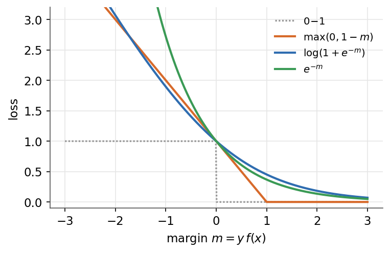+	*Pertes basées sur la marge, chacune un substitut convexe de la perte 0-1 qui pénalise les marges faibles ou négatives.*
+
+	## Descente de gradient
+
+	### Règle de mise à jour
+
+	La descente de gradient déplace itérativement les paramètres $\theta$ à l'opposé du gradient du coût, mis à l'échelle par un taux d'apprentissage $\alpha > 0$ :
+
+	$$\boxed{\,\theta \leftarrow \theta - \alpha\,\nabla_\theta J(\theta)\,}$$
+
+	Le gradient pointe dans la direction de plus forte croissance, donc avancer à son opposé fait décroître $J$. Le pas $\alpha$ contrôle l'ampleur de chaque mise à jour.
+
+	*Remarque :* si $\alpha$ est trop grand les itérés peuvent diverger, s'il est trop petit la convergence est lente.
+
+	### Par lots ou stochastique
+
+	Les deux variantes diffèrent par le nombre d'exemples contribuant à une mise à jour.
+
+	| Variante | Exemples par mise à jour | Mise à jour |
+	| --- | --- | --- |
+	| Par lots | Tous les $m$ | $\theta \leftarrow \theta - \alpha\,\nabla_\theta J(\theta)$ |
+	| Stochastique (SGD) | Un seul $(x^{(i)}, y^{(i)})$ | $\theta \leftarrow \theta - \alpha\,\nabla_\theta L\!\left(h_\theta(x^{(i)}), y^{(i)}\right)$ |
+
+	Le mode par lots donne une descente lisse mais lit tout l'ensemble à chaque pas. SGD met à jour après chaque exemple, donc peu coûteux par pas et bruité.
+
+	### Mise à jour LMS (Widrow-Hoff)
+
+	Pour l'erreur quadratique, la mise à jour stochastique par coordonnée est définie comme :
+
+	$$\boxed{\,\theta_j \leftarrow \theta_j + \alpha\left(y^{(i)} - h_\theta(x^{(i)})\right)x_j^{(i)}\,}$$
+
+	La correction est proportionnelle au résidu $y^{(i)} - h_\theta(x^{(i)})$ multiplié par la composante $x_j^{(i)}$.
+
+	*Remarque :* un grand résidu produit un grand pas, une prédiction correcte ne produit aucune mise à jour.
+
+	
+
+	*La descente de gradient descend la pente vers le minimum (étoile).*
+
+	## Vraisemblance et estimation du maximum de vraisemblance
+
+	### Vraisemblance
+
+	La vraisemblance $L(\theta)$ est définie comme la probabilité des cibles observées sous le modèle, vue comme une fonction des paramètres $\theta$. En supposant les exemples indépendants, elle se factorise :
+
+	$$\boxed{\,L(\theta)=\prod_{i=1}^{m} p\!\left(y^{(i)} \mid x^{(i)}; \theta\right)\,}$$
+
+	### Log-vraisemblance
+
+	Les produits sont malcommodes à optimiser, on prend donc le logarithme. La log-vraisemblance $\ell(\theta)$ est définie comme :
+
+	$$\boxed{\,\ell(\theta)=\sum_{i=1}^{m} \log p\!\left(y^{(i)} \mid x^{(i)}; \theta\right)\,}$$
+
+	Le $\log$ est monotone, il a donc le même maximiseur que $L(\theta)$ tout en transformant le produit en somme.
+
+	### Estimation du maximum de vraisemblance
+
+	Le maximum de vraisemblance est défini comme la valeur des paramètres qui rend les données les plus probables :
+
+	$$\boxed{\,\theta_{\mathrm{MLE}}=\arg\max_\theta\,\ell(\theta)\,}$$
+
+	*Remarque :* maximiser la log-vraisemblance équivaut à minimiser le coût $J(\theta) = -\ell(\theta)$. C'est exactement la vue par minimisation du coût des leçons précédentes, vraisemblance et coût sont donc deux faces d'un même objectif.
+
+	## Algorithme de Newton
+
+	### Mise à jour unidimensionnelle
+
+	Pour trouver un point stationnaire de la log-vraisemblance, l'algorithme de Newton suit l'approximation quadratique locale. La mise à jour scalaire est définie comme :
+
+	$$\boxed{\,\theta \leftarrow \theta - \frac{\ell'(\theta)}{\ell''(\theta)}\,}$$
+
+	Elle divise la dérivée première par la dérivée seconde, donc le pas s'adapte automatiquement à la courbure.
+
+	### Mise à jour multivariée
+
+	Avec un vecteur de paramètres $\theta \in \mathbb{R}^{n+1}$, la dérivée seconde devient la matrice hessienne $H$, avec $H_{jk}=\dfrac{\partial^2 \ell}{\partial\theta_j\,\partial\theta_k}$. La mise à jour est définie comme :
+
+	$$\boxed{\,\theta \leftarrow \theta - H^{-1}\,\nabla_\theta \ell(\theta)\,}$$
+
+	*Remarque :* chaque pas résout un système linéaire en $H$, une opération en $O(n^3)$, donc l'algorithme de Newton est coûteux quand le nombre de variables $n$ est grand.
+
+	### Newton ou descente de gradient
+
+	| Propriété | Algorithme de Newton | Descente de gradient |
+	| --- | --- | --- |
+	| Ordre | Second (utilise la courbure $H$) | Premier (utilise le gradient seul) |
+	| Coût par pas | Élevé ($O(n^3)$, inverse $H$) | Faible ($O(n)$ par exemple) |
+	| Convergence | Quadratique près de l'optimum, peu de pas | Linéaire, beaucoup de pas |
+	| Réglage | Aucun taux d'apprentissage | Nécessite un taux $\alpha$ |
+
+	*Remarque :* l'algorithme de Newton converge en très peu d'itérations mais paie un coût élevé par pas, donc la descente de gradient est préférée quand $n$ est grand.
+
+	*Ces outils sont indépendants du modèle. La partie suivante les applique à la classe d'hypothèses la plus simple, où la prédiction est une fonction linéaire des variables : les modèles linéaires.*
+
+	---
+	Suivant : [Modèles linéaires](/fr/Machine%20Learning/03%20Linear%20models) · [Vue d'ensemble du cours](/fr/Machine%20Learning)
/dev/null .. fr/Machine Learning/02 General concepts/gradient-descent.png
/dev/null .. fr/Machine Learning/02 General concepts/loss-functions.png
/dev/null .. fr/Machine Learning/03 Linear models.md
@@ 0,0 1,193 @@
+	# Modèles linéaires
+
+	Les modèles linéaires prédisent à partir d'un score linéaire $\theta^T x$. Ce module couvre la régression linéaire (cibles continues), la régression logistique (classification binaire) et le cadre des modèles linéaires généralisés qui unifie les deux via la famille exponentielle. Chaque modèle est ajusté par maximum de vraisemblance et partage la même mise à jour par gradient.
+
+	**Objectifs**
+	- Définir l'hypothèse linéaire et ajuster $\theta$ par la mise à jour LMS ou par l'équation normale en forme close.
+	- Comprendre pourquoi les moindres carrés sont l'estimation du maximum de vraisemblance sous bruit gaussien.
+	- Transformer le score linéaire en probabilité via la sigmoïde et l'ajuster par montée de gradient ou méthode de Newton.
+	- Classer avec le perceptron et savoir quand sa règle d'apprentissage converge.
+	- Reconnaître la forme de la famille exponentielle et construire un MLG à partir de ses trois hypothèses.
+	- Retrouver les régressions linéaire, logistique et softmax comme cas particuliers.
+
+	## Régression linéaire
+
+	### Hypothèse
+
+	L'hypothèse est linéaire en l'entrée augmentée $x \in \mathbb{R}^{n+1}$ avec $x_0 = 1$ et les paramètres $\theta \in \mathbb{R}^{n+1}$ :
+
+	$$\boxed{ h_\theta(x) = \theta^T x }$$
+
+	### Fonction de coût
+
+	Le coût est défini comme la demi-somme des carrés des résidus sur les $m$ exemples :
+
+	$$\boxed{ J(\theta) = \tfrac{1}{2}\sum_{i=1}^{m}\left(h_\theta(x^{(i)}) - y^{(i)}\right)^2 }$$
+
+	### Mise à jour LMS
+
+	La descente de gradient sur $J$ donne la mise à jour des moindres carrés moyens (Widrow-Hoff), appliquée par exemple $(x^{(i)}, y^{(i)})$ :
+
+	$$\boxed{ \theta_j \leftarrow \theta_j + \alpha\left(y^{(i)} - h_\theta(x^{(i)})\right)x_j^{(i)} }$$
+
+	avec un taux d'apprentissage $\alpha > 0$.
+
+	| variante | règle de mise à jour | par étape | à utiliser quand |
+	| --- | --- | --- | --- |
+	| GD par lots | somme sur les $m$ exemples | $O(mn)$ | $m$ petit à modéré |
+	| GD stochastique (SGD) | un exemple à la fois | $O(n)$ | $m$ grand, flux de données |
+
+	### Équation normale
+
+	Annuler $\nabla_\theta J(\theta) = 0$ donne une solution en forme close à partir de la matrice de conception $X$ et du vecteur cible $y$ :
+
+	$$\boxed{ \theta = (X^T X)^{-1}X^T y }$$
+
+	*Remarque :* l'équation normale ne demande ni taux d'apprentissage ni itération, mais inverser $X^T X$ coûte $O(n^3)$, donc pour $n$ grand la mise à jour itérative LMS est préférée.
+
+	### Interprétation probabiliste
+
+	Supposons $y^{(i)} = \theta^T x^{(i)} + \varepsilon^{(i)}$ avec un bruit gaussien i.i.d. $\varepsilon^{(i)} \sim \mathcal{N}(0, \sigma^2)$. Maximiser la log-vraisemblance revient alors à minimiser le coût des moindres carrés :
+
+	$$\boxed{ \arg\max_\theta \ell(\theta) = \arg\min_\theta J(\theta) }$$
+
+	*Remarque :* c'est pourquoi les moindres carrés sont un objectif fondé et pas seulement commode.
+
+	
+
+	*Les moindres carrés ajustent la droite qui minimise les résidus au carré (segments gris).*
+
+	## Régression logistique
+
+	### Sigmoïde
+
+	La fonction sigmoïde (logistique) comprime un score brut $z \in \mathbb{R}$ en une probabilité :
+
+	$$\boxed{ g(z) = \frac{1}{1 + e^{-z}} \in (0, 1) }$$
+
+	Sa dérivée a la forme commode $g'(z) = g(z)\left(1 - g(z)\right)$.
+
+	### Modèle
+
+	L'hypothèse renvoie la probabilité de la classe positive, $\phi$ étant la probabilité prédite :
+
+	$$\boxed{ \phi = h_\theta(x) = g(\theta^T x) = p(y = 1 \mid x; \theta) }$$
+
+	Les étiquettes valent $y \in \{0, 1\}$, donc la loi conditionnelle est de Bernoulli :
+
+	$$\boxed{ p(y \mid x; \theta) = \phi^{y}(1 - \phi)^{1 - y} }$$
+
+	### Log-vraisemblance
+
+	Sur $m$ exemples i.i.d. la log-vraisemblance est l'opposé de l'entropie croisée sommée sur les données :
+
+	$$\boxed{ \ell(\theta) = \sum_{i=1}^{m}\left[ y^{(i)}\log \phi^{(i)} + (1 - y^{(i)})\log(1 - \phi^{(i)}) \right] }$$
+
+	avec $\phi^{(i)} = h_\theta(x^{(i)})$.
+
+	### Montée de gradient
+
+	Maximiser $\ell$ par montée de gradient donne la même forme que la mise à jour LMS :
+
+	$$\boxed{ \theta_j \leftarrow \theta_j + \alpha\left(y^{(i)} - h_\theta(x^{(i)})\right)x_j^{(i)} }$$
+
+	*Remarque :* la mise à jour a la même forme que la régression linéaire, bien que $h_\theta$ soit maintenant la sigmoïde. Ce n'est pas un hasard, les deux sont des modèles linéaires généralisés.
+
+	### Méthode de Newton
+
+	La méthode de Newton converge plus vite près de l'optimum. En une dimension :
+
+	$$\boxed{ \theta \leftarrow \theta - \frac{\ell'(\theta)}{\ell''(\theta)} }$$
+
+	Dans le cas vectoriel elle utilise la hessienne $H$ de $\ell$ :
+
+	$$\boxed{ \theta \leftarrow \theta - H^{-1}\nabla_\theta \ell(\theta) }$$
+
+	*Remarque :* la régression logistique n'a pas de solution en forme close pour $\theta$, elle est donc toujours ajustée itérativement (montée de gradient ou Newton).
+
+	
+
+	*À gauche : la sigmoïde envoie les scores dans l'intervalle (0,1). À droite : la frontière de décision et la probabilité prédite.*
+
+	## Perceptron
+
+	Le perceptron est le premier classifieur linéaire. Il conserve le score linéaire $\theta^T x$ de la régression logistique mais remplace la sigmoïde par un seuil dur, donc la sortie est une étiquette de classe et non une probabilité. Les étiquettes valent $y \in \{0, 1\}$.
+
+	### Activation et hypothèse
+
+	L'activation est la fonction échelon :
+
+	$$\boxed{ g(z) = \begin{cases} 1 & \text{si } z \ge 0 \\ 0 & \text{sinon} \end{cases} }$$
+
+	et l'hypothèse l'applique au score linéaire :
+
+	$$\boxed{ h_\theta(x) = g(\theta^T x) }$$
+
+	### Règle d'apprentissage
+
+	Le perceptron est entraîné en ligne, un exemple à la fois, et ne corrige $\theta$ que sur un point mal classé :
+
+	$$\boxed{ \theta_j \leftarrow \theta_j + \alpha\left(y^{(i)} - h_\theta(x^{(i)})\right)x_j^{(i)} }$$
+
+	*Remarque :* c'est la même forme que la mise à jour LMS et que la montée de gradient logistique. Seule l'activation $g$ change (identité, sigmoïde, échelon). Quand la prédiction est correcte, le facteur $y^{(i)} - h_\theta(x^{(i)})$ est nul, donc les points bien classés laissent $\theta$ inchangé.
+
+	
+
+	*Le perceptron trouve un hyperplan séparateur. Ce n'est pas nécessairement celui à marge maximale que choisira le SVM.*
+
+	### Convergence
+
+	| données | comportement |
+	| --- | --- |
+	| linéairement séparables | converge en un nombre fini de mises à jour |
+	| non séparables | ne converge jamais, les poids oscillent |
+
+	*Remarque :* le perceptron s'arrête au premier hyperplan qui sépare les données, généralement pas celui à la marge la plus large. Cet écart motive la machine à vecteurs de support (qui maximise la marge) et, empilé en couches, le réseau de neurones (un perceptron est une unité).
+
+	## Modèles linéaires généralisés
+
+	### Famille exponentielle
+
+	Une distribution appartient à la famille exponentielle si sa densité s'écrit avec le paramètre naturel $\eta$, la statistique suffisante $T(y)$, la log-partition $a(\eta)$ et la mesure de base $b(y)$ :
+
+	$$\boxed{ p(y; \eta) = b(y)\exp\left(\eta\, T(y) - a(\eta)\right) }$$
+
+	### Hypothèses du MLG
+
+	Un MLG repose sur trois choix. La réponse appartient à la famille exponentielle, le paramètre naturel est linéaire en l'entrée, et la prédiction est la statistique suffisante espérée :
+
+	$$\boxed{ \eta = \theta^T x }$$
+
+	$$\boxed{ h_\theta(x) = \mathbb{E}\left[T(y) \mid x; \theta\right] }$$
+
+	### Tableau des familles
+
+	| Distribution | $\eta$ | $T(y)$ | $a(\eta)$ | $b(y)$ |
+	| --- | --- | --- | --- | --- |
+	| Bernoulli | $\log\dfrac{\phi}{1-\phi}$ | $y$ | $\log(1 + e^{\eta})$ | $1$ |
+	| Gaussienne ($\sigma^2 = 1$) | $\mu$ | $y$ | $\tfrac{1}{2}\eta^2$ | $\dfrac{1}{\sqrt{2\pi}}e^{-y^2/2}$ |
+	| Poisson | $\log\lambda$ | $y$ | $e^{\eta}$ | $\dfrac{1}{y!}$ |
+	| Géométrique | $\log(1-\phi)$ | $y$ | $\log\dfrac{e^{\eta}}{1 - e^{\eta}}$ | $1$ |
+
+	*Remarque :* pour la Bernoulli, $\eta$ est le log-rapport de cotes et son inverse est la sigmoïde, $\phi = g(\eta)$. C'est pourquoi la régression logistique a cette forme.
+
+	### Régression softmax
+
+	Pour des étiquettes multiclasses $y \in \{1, \dots, k\}$ le MLG donne la régression softmax, avec un vecteur de paramètres $\theta_k$ par classe :
+
+	$$\boxed{ p(y = k \mid x; \theta) = \frac{\exp(\theta_k^T x)}{\sum_{j}\exp(\theta_j^T x)} }$$
+
+	### Recette du MLG
+
+	```mermaid
+	graph TD
+	A["choisir une distribution de reponse"] --> B["l ecrire en forme de famille exponentielle"]
+	B --> C["poser le parametre naturel eta lineaire en x"]
+	C --> D["la prediction est la statistique suffisante esperee"]
+	D --> E["ajuster theta par maximum de vraisemblance"]
+	```
+
+	*Les modèles linéaires, y compris le perceptron, se contentent d'une frontière qui sépare les classes. La partie suivante cherche la meilleure : la machine à vecteurs de support maximise la marge.*
+
+	---
+	Suivant : [Machines à vecteurs de support](/fr/Machine%20Learning/04%20Support%20Vector%20Machines) · [Vue d'ensemble du cours](/fr/Machine%20Learning)
/dev/null .. fr/Machine Learning/03 Linear models/linear-regression.png
/dev/null .. fr/Machine Learning/03 Linear models/logistic-regression.png
/dev/null .. fr/Machine Learning/03 Linear models/perceptron.png
/dev/null .. fr/Machine Learning/04 Support Vector Machines.md
@@ 0,0 1,222 @@
+	# Machines à vecteurs de support
+
+	Les machines à vecteurs de support sont des classifieurs linéaires à grande marge. Elles
+	choisissent la frontière qui maximise la distance aux points les plus proches, contrôlent le
+	surapprentissage avec la perte charnière et une pénalité $C$, et utilisent des noyaux pour
+	ajuster des frontières non linéaires sans jamais former l'application de caractéristiques. Partout,
+	les étiquettes valent $y \in \{-1,+1\}$ et la décision utilise un score brut $z = w^T x - b$.
+
+	**Objectifs**
+	- Définir l'hypothèse SVM, son hyperplan séparateur et la marge géométrique.
+	- Formuler le primal à marge dure et le primal à marge souple avec perte charnière et pénalité $C$.
+	- Définir les noyaux, l'astuce du noyau et la condition de Mercer.
+	- Former le lagrangien, dériver le dual et les conditions KKT, et définir les vecteurs de support.
+
+	## Classifieur à marge optimale
+
+	Les étiquettes valent $y \in \{-1,+1\}$, avec un vecteur de poids $w \in \mathbb{R}^{n}$ et un biais $b$.
+
+	### Hypothèse et frontière
+
+	L'hypothèse est définie comme le signe du score brut $z = w^T x - b$ :
+
+	$$\boxed{ h(x) = \operatorname{sign}(w^T x - b) }$$
+
+	La frontière de décision est l'ensemble des points de score nul :
+
+	$$\boxed{ w^T x - b = 0 }$$
+
+	*Remarque :* $w$ est orthogonal à la frontière, il en fixe donc l'orientation, et $b$ fixe le décalage.
+
+	### Marge géométrique
+
+	La marge géométrique de l'exemple $i$ est définie comme sa distance signée à la frontière, rendue
+	positive par l'étiquette :
+
+	$$\boxed{ \gamma^{(i)} = y^{(i)} \, \frac{w^T x^{(i)} - b}{\lVert w \rVert} }$$
+
+	Un point correctement classé vérifie $\gamma^{(i)} > 0$. La marge du jeu de données est la plus
+	petite $\gamma^{(i)}$ sur tous les exemples.
+
+	*Remarque :* diviser par $\lVert w \rVert$ rend la marge invariante au rééchelonnement de $(w,b)$,
+	contrairement au score brut $z$.
+
+	### Primal à marge dure
+
+	En fixant l'échelle pour que les points les plus proches vérifient $y^{(i)}(w^T x^{(i)} - b) = 1$,
+	maximiser la marge équivaut à minimiser $\lVert w \rVert^2$ sous une marge fonctionnelle unitaire :
+
+	$$\boxed{ \min_{w,b} \tfrac{1}{2}\lVert w \rVert^2 \quad \text{s.c.} \quad y^{(i)}(w^T x^{(i)} - b) \ge 1 \ \ \forall i }$$
+
+	C'est un programme quadratique convexe à contraintes linéaires, il admet donc un optimum unique.
+
+	*Remarque :* il exige des données linéairement séparables. La leçon suivante assouplit cela avec
+	des variables d'écart.
+
+	
+
+	*L'hyperplan optimal (trait plein) maximise la marge (pointillés). Les points entourés sont les vecteurs de support.*
+
+	## Perte charnière
+
+	Le score brut est $z = w^T x - b$ et les étiquettes valent $y \in \{-1,+1\}$.
+
+	### Perte charnière
+
+	La perte charnière est définie comme l'écart par lequel la marge $yz$ tombe sous $1$, tronqué à zéro :
+
+	$$\boxed{ L(z,y) = \max(0,\, 1 - yz), \quad z = w^T x - b }$$
+
+	Elle est nulle dès que $yz \ge 1$ (le point est correct et au-delà de la marge) et croît
+	linéairement à l'intérieur ou au-delà de la marge.
+
+	*Remarque :* la perte charnière est convexe mais non dérivable en $yz = 1$, on l'optimise donc
+	avec des sous-gradients.
+
+	### Primal à marge souple
+
+	On introduit un écart $\xi_i \ge 0$ par exemple pour autoriser les violations de marge, pénalisé
+	par $C > 0$ :
+
+	$$\boxed{ \min_{w,b,\xi} \tfrac{1}{2}\lVert w \rVert^2 + C\sum_{i=1}^{m}\xi_i \quad \text{s.c.} \quad y^{(i)}(w^T x^{(i)} - b) \ge 1 - \xi_i, \ \ \xi_i \ge 0 }$$
+
+	À l'optimum $\xi_i = \max(0,\, 1 - y^{(i)}(w^T x^{(i)} - b))$, donc éliminer les écarts donne la
+	forme régularisée sans contrainte :
+
+	$$\boxed{ \min_{w,b} \tfrac{1}{2}\lVert w \rVert^2 + C\sum_{i=1}^{m}\max\!\big(0,\, 1 - y^{(i)}(w^T x^{(i)} - b)\big) }$$
+
+	C'est de la régularisation plus une perte charnière : le terme $\tfrac{1}{2}\lVert w \rVert^2$
+	élargit la marge et la somme pénalise les violations.
+
+	### Rôle de $C$
+
+	| $C$ | Pénalité des violations | Marge | Comportement |
+	| --- | --- | --- | --- |
+	| petit | faible | large | plus de violations tolérées, variance plus faible |
+	| grand | forte | étroite | moins de violations, ajuste davantage les données |
+
+	*Remarque :* quand $C \to \infty$ aucune violation n'est tolérée, ce qui redonne le classifieur à
+	marge dure.
+
+	## Noyaux
+
+	### Définition d'un noyau
+
+	Un noyau est défini comme le produit scalaire d'une application de caractéristiques $\phi$
+	appliquée à deux entrées :
+
+	$$\boxed{ K(x,z) = \phi(x)^T \phi(z) }$$
+
+	Un noyau valide calcule ce produit scalaire directement, donc $\phi$ n'a jamais à être formée
+	(elle peut même être de dimension infinie).
+
+	### Astuce du noyau
+
+	Le dual du SVM ne dépend des données qu'à travers des produits scalaires
+	$\langle x^{(i)}, x^{(j)} \rangle$. L'astuce du noyau remplace chaque produit scalaire par un noyau :
+
+	$$\boxed{ \langle x^{(i)}, x^{(j)} \rangle \ \longrightarrow \ K(x^{(i)}, x^{(j)}) }$$
+
+	Cela ajuste une frontière linéaire dans l'espace de caractéristiques, donc non linéaire dans
+	l'espace d'origine, au prix d'évaluer $K$ au lieu de $\phi$.
+
+	Un choix très répandu est le noyau gaussien (RBF) :
+
+	$$\boxed{ K(x,z) = \exp\!\left( -\frac{\lVert x - z \rVert^2}{2\sigma^2} \right) }$$
+
+	### Condition de Mercer
+
+	Une fonction $K$ est un noyau valide si et seulement si, pour tout échantillon fini, sa matrice de
+	Gram est symétrique semi-définie positive :
+
+	$$\boxed{ K = K^T, \qquad K \succeq 0 }$$
+
+	*Remarque :* c'est la condition de Mercer. Elle garantit l'existence d'une application $\phi$, donc
+	le dual reste convexe.
+
+	### Noyaux usuels
+
+	| Noyau | $K(x,z)$ | Note |
+	| --- | --- | --- |
+	| Linéaire | $x^T z$ | pas d'application, redonne le SVM linéaire |
+	| Polynomial | $(x^T z + c)^d$ | degré $d$, décalage $c$ |
+	| Gaussien (RBF) | $\exp\!\big(-\tfrac{\lVert x - z \rVert^2}{2\sigma^2}\big)$ | dimension infinie, local |
+
+	*Remarque :* un petit $\sigma$ rend le noyau RBF très local, ce qui peut surapprendre. Il se règle
+	en compromis avec $C$.
+
+	
+
+	*Un noyau RBF sépare des classes non linéairement séparables, par une frontière non linéaire dans l'espace d'entrée.*
+
+	## Lagrangien et dualité
+
+	### Lagrangien
+
+	Pour un objectif primal $f(w)$ avec contraintes d'inégalité $g_i(w) \le 0$ et multiplicateurs
+	$\beta_i \ge 0$, le lagrangien est défini comme :
+
+	$$\boxed{ \mathcal{L}(w,\beta) = f(w) + \sum_{i=1}^{m} \beta_i \, g_i(w) }$$
+
+	Appliqué au primal SVM $\tfrac{1}{2}\lVert w \rVert^2$ avec contraintes
+	$1 - y^{(i)}(w^T x^{(i)} - b) \le 0$, les conditions de stationnarité $\nabla_w \mathcal{L} = 0$ et
+	$\partial_b \mathcal{L} = 0$ donnent :
+
+	$$\boxed{ w = \sum_{i=1}^{m} \beta_i\, y^{(i)} x^{(i)}, \qquad \sum_{i=1}^{m} \beta_i\, y^{(i)} = 0 }$$
+
+	Le $w$ optimal est donc une combinaison linéaire des entrées d'apprentissage pondérées par
+	$\beta_i y^{(i)}$.
+
+	### Problème dual
+
+	En réinjectant ces relations, on élimine $w$ et $b$, ce qui laisse un problème en $\beta$ ne
+	dépendant des données qu'à travers des produits scalaires :
+
+	$$\boxed{ \max_{\beta} \ \sum_{i=1}^{m}\beta_i - \tfrac{1}{2}\sum_{i,j}\beta_i \beta_j\, y^{(i)} y^{(j)} \langle x^{(i)}, x^{(j)} \rangle \quad \text{s.c.} \quad \beta_i \ge 0, \ \ \sum_{i}\beta_i y^{(i)} = 0 }$$
+
+	Les produits scalaires sont exactement l'endroit où l'on substitue un noyau $K$ (voir [Noyaux](/fr/Machine%20Learning/04%20Support%20Vector%20Machines#noyaux)).
+
+	### KKT et vecteurs de support
+
+	À l'optimum, l'écart complémentaire lie chaque multiplicateur à sa contrainte :
+
+	$$\boxed{ \beta_i \big[\, y^{(i)}(w^T x^{(i)} - b) - 1 \,\big] = 0 }$$
+
+	Les vecteurs de support sont définis comme les exemples à multiplicateur non nul :
+
+	$$\boxed{ \text{vecteurs de support} = \{\, i : \beta_i > 0 \,\} }$$
+
+	Ce sont les points exactement sur la marge. Tous les autres ont $\beta_i = 0$ et n'influencent pas
+	$w$.
+
+	### Décision à noyau
+
+	Remplacer le produit scalaire par un noyau donne une règle de décision exprimée uniquement à
+	travers les vecteurs de support :
+
+	$$\boxed{ h(x) = \operatorname{sign}\!\left( \sum_{i=1}^{m} \beta_i\, y^{(i)}\, K(x^{(i)}, x) - b \right) }$$
+
+	*Remarque :* seuls les vecteurs de support ($\beta_i > 0$) contribuent, donc le coût de prédiction
+	croît avec leur nombre, pas avec $m$.
+
+	### Du primal à la décision
+
+	```mermaid
+	flowchart TD
+	A["QP primal : minimiser demi norme au carre"]
+	B["lagrangien avec multiplicateurs"]
+	C["probleme dual en beta"]
+	D["conditions KKT"]
+	E["vecteurs de support : beta superieur a zero"]
+	F["regle de decision a noyau"]
+	A --> B
+	B --> C
+	C --> D
+	D --> E
+	E --> F
+	```
+
+	*Les machines à vecteurs de support tracent une seule frontière, éventuellement à noyau. La dernière partie suit une autre voie : découper l'espace des variables par des règles simples et combiner de nombreux modèles en un ensemble.*
+
+	---
+	Suivant : [Arbres de décision et méthodes d'ensemble](/fr/Machine%20Learning/05%20Decision%20trees%20and%20ensemble%20methods) · [Vue d'ensemble du cours](/fr/Machine%20Learning)
/dev/null .. fr/Machine Learning/04 Support Vector Machines/svm-kernel.png
/dev/null .. fr/Machine Learning/04 Support Vector Machines/svm-margin.png
/dev/null .. fr/Machine Learning/05 Decision trees and ensemble methods.md
@@ 0,0 1,181 @@
+	# Arbres de décision et méthodes d'ensemble
+
+	Les modèles d'arbre partitionnent l'espace d'entrée en régions alignées sur les axes et ajustent une constante par région, ce qui donne des prédicteurs interprétables mais à forte variance. Les méthodes d'ensemble combinent plusieurs arbres : le bagging et les forêts aléatoires moyennent des arbres construits indépendamment pour réduire la variance, tandis que le boosting construit les arbres de façon séquentielle pour réduire le biais.
+
+	**Objectifs**
+	- Exprimer un arbre comme une fonction constante par morceaux et choisir les coupures avec un critère d'impureté.
+	- Contrôler le surapprentissage par l'élagage à complexité coûteuse.
+	- Réduire la variance par le bagging et décorréler les arbres via le sous-échantillonnage des variables.
+	- Estimer gratuitement l'erreur de généralisation avec les échantillons hors-sac.
+	- Construire un prédicteur fort comme somme additive d'apprenants faibles (AdaBoost, gradient boosting).
+
+	## Arbres de décision CART
+
+	### L'arbre comme partition
+
+	Un arbre CART partitionne l'espace d'entrée en $M$ régions disjointes $R_1,\dots,R_M$ (les feuilles) et prédit une constante $c_m$ sur chacune. La prédiction est définie par
+
+	$$\boxed{ h(x)=\sum_{m=1}^{M} c_m\,\mathbf{1}\{x\in R_m\} }$$
+
+	Chaque nœud interne teste une variable contre un seuil, $x_j\le s$, envoyant un exemple à gauche ou à droite. Un chemin de la racine à une feuille est une conjonction de tels tests.
+
+	*Remarque :* les régions sont des boîtes alignées sur les axes, donc la frontière de décision est en escalier. Un arbre seul a un faible biais mais une forte variance.
+
+	### Impureté et choix de la coupure
+
+	Pour une région de proportions de classes $\hat p_k$, l'impureté mesure le mélange des étiquettes. L'indice de Gini est défini par
+
+	$$\boxed{ G = 1-\sum_{k}\hat p_k^{\,2} }$$
+
+	et l'entropie par
+
+	$$\boxed{ H = -\sum_{k}\hat p_k\log_2\hat p_k }$$
+
+	Une coupure candidate envoie $N_-$ exemples vers l'enfant $R_-$ et $N_+$ vers $R_+$ sur $N$ au total. Son gain d'information est défini par
+
+	$$\boxed{ IG = I(\text{parent})-\frac{N_-}{N}\,I(R_-)-\frac{N_+}{N}\,I(R_+) }$$
+
+	où $I$ est l'impureté choisie. CART retient gloutonnement la variable et le seuil qui maximisent $IG$ à chaque nœud.
+
+	| critère | formule | plage (binaire) | note |
+	| --- | --- | --- | --- |
+	| Gini | $1-\sum_k\hat p_k^{2}$ | $[0,0.5]$ | moins coûteux, sans logarithme |
+	| entropie | $-\sum_k\hat p_k\log_2\hat p_k$ | $[0,1]$ | théorie de l'information |
+
+	*Remarque :* les deux critères choisissent presque toujours la même coupure. Gini est le défaut de la plupart des implémentations car il évite le logarithme.
+
+	### Arbres de régression
+
+	En régression, la valeur de la feuille est la moyenne des cibles dans la région, définie par
+
+	$$\boxed{ c_m=\frac{1}{N_m}\sum_{x^{(i)}\in R_m} y^{(i)} }$$
+
+	et les coupures minimisent l'erreur quadratique intra-région plutôt qu'une impureté de classification.
+
+	### Élagage
+
+	Un arbre non élagué ajuste exactement l'ensemble d'entraînement et surapprend. L'élagage à complexité coûteuse arbitre entre l'ajustement et la taille de l'arbre $|T|$ (le nombre de feuilles) via une pénalité $\alpha\ge0$ :
+
+	$$\boxed{ C_\alpha(T)=\sum_{m} N_m\,I(R_m)+\alpha\,|T| }$$
+
+	Augmenter $\alpha$ effondre les coupures les plus faibles, produisant une suite emboîtée de sous-arbres. Le meilleur $\alpha$ est choisi par validation croisée.
+
+	```mermaid
+	graph TD
+	A["x_j <= s ?"] -->|"oui"| B["x_k <= t ?"]
+	A -->|"non"| C["feuille R3"]
+	B -->|"oui"| D["feuille R1"]
+	B -->|"non"| E["feuille R2"]
+	```
+
+	
+
+	*Un arbre découpe l'espace en régions alignées sur les axes, chacune à prédiction constante.*
+
+	## Forêts aléatoires
+
+	### Bagging
+
+	Le bagging (bootstrap aggregating) entraîne $B$ arbres sur $B$ rééchantillons bootstrap des données et les moyenne. Le prédicteur agrégé est défini par
+
+	$$\boxed{ h_{\text{bag}}(x)=\frac{1}{B}\sum_{b=1}^{B} h_b(x) }$$
+
+	En classification, la moyenne est remplacée par un vote majoritaire. Moyenner laisse le biais inchangé tout en réduisant la variance.
+
+	Un échantillon bootstrap tire $N$ exemples avec remise parmi $N$ exemples. La probabilité qu'un exemple donné ne soit jamais tiré vaut $(1-\tfrac1N)^N\to e^{-1}\approx0{,}37$, donc environ 37 % des données restent hors de chaque arbre. Ce sont ses exemples hors-sac (OOB).
+
+	### Variance d'une moyenne
+
+	Si les $B$ arbres ont chacun une variance $\sigma^2$ et une corrélation deux à deux $\rho$, la variance de leur moyenne vaut
+
+	$$\boxed{ \rho\sigma^2+\frac{1-\rho}{B}\,\sigma^2 }$$
+
+	Le second terme s'annule quand $B$ croît, mais le premier, $\rho\sigma^2$, persiste. Réduire la corrélation $\rho$ entre les arbres est donc le levier clé, et c'est précisément ce que visent les forêts aléatoires.
+
+	### Forêts aléatoires
+
+	Une forêt aléatoire est du bagging avec sous-échantillonnage des variables : à chaque coupure, seul un sous-ensemble aléatoire de $m_{\text{try}}$ variables est considéré comme candidat. Les choix usuels sont
+
+	$$\boxed{ m_{\text{try}}=\lfloor\sqrt{n}\,\rfloor\ \text{(classification)},\qquad m_{\text{try}}=\lfloor n/3\rfloor\ \text{(régression)} }$$
+
+	Restreindre les variables candidates empêche tous les arbres de couper sur la même variable dominante, ce qui décorrèle les arbres et abaisse $\rho$.
+
+	*Remarque :* l'erreur OOB moyenne l'erreur de chaque arbre uniquement sur les exemples qu'il n'a jamais vus, donnant une estimation proche d'une validation croisée sans coût supplémentaire.
+
+	| propriété | bagging | forêt aléatoire |
+	| --- | --- | --- |
+	| rééchantillonnage | bootstrap | bootstrap |
+	| variables candidates | les $n$ variables | $m_{\text{try}}$ variables aléatoires |
+	| corrélation des arbres $\rho$ | plus élevée | plus faible |
+	| réduction de variance | modérée | plus forte |
+
+	```mermaid
+	graph TD
+	A["jeu d'entrainement"] --> B1["echantillon bootstrap 1"]
+	A --> B2["echantillon bootstrap 2"]
+	A --> B3["echantillon bootstrap B"]
+	B1 --> T1["arbre 1"]
+	B2 --> T2["arbre 2"]
+	B3 --> T3["arbre B"]
+	T1 --> AGG["agregation : moyenne ou vote"]
+	T2 --> AGG
+	T3 --> AGG
+	```
+
+	
+
+	*(a) Un arbre profond seul surajuste avec une frontière en escalier. (b) Une forêt aléatoire moyenne de nombreux arbres pour une frontière plus lisse.*
+
+	## Boosting
+
+	### Modèle additif
+
+	Le boosting construit un prédicteur comme une somme pondérée de $T$ apprenants faibles $h_t$ (typiquement des arbres peu profonds), ajustés un à un. Le modèle additif est défini par
+
+	$$\boxed{ H_T(x)=\sum_{t=1}^{T}\alpha_t\,h_t(x) }$$
+
+	Chaque étape corrige les erreurs de la somme courante, donc l'ensemble est construit de façon séquentielle et réduit le biais plutôt que la variance.
+
+	### AdaBoost
+
+	Avec des étiquettes $y\in\{-1,+1\}$, AdaBoost conserve des poids d'exemples $w^{(i)}$ qui se concentrent sur les points actuellement mal classés. Au tour $t$, l'apprenant faible a une erreur pondérée $\varepsilon_t$, et son coefficient est défini par
+
+	$$\boxed{ \alpha_t=\tfrac12\log\frac{1-\varepsilon_t}{\varepsilon_t} }$$
+
+	ainsi un apprenant plus précis ($\varepsilon_t$ petit) obtient un vote plus grand. Les poids sont ensuite mis à jour par
+
+	$$\boxed{ w^{(i)}\leftarrow w^{(i)}\exp\!\big(-\alpha_t\,y^{(i)}h_t(x^{(i)})\big) }$$
+
+	puis renormalisés. Les exemples mal classés ($y^{(i)}h_t(x^{(i)})<0$) gagnent du poids, donc l'apprenant suivant se concentre sur eux.
+
+	### Gradient boosting
+
+	Le gradient boosting généralise l'idée à toute perte différentiable $L$. À l'étape $t$, il ajuste l'apprenant suivant sur l'opposé du gradient de la perte évalué au modèle courant, le pseudo-résidu défini par
+
+	$$\boxed{ r^{(i)}_t=-\left[\frac{\partial L\big(y^{(i)},f(x^{(i)})\big)}{\partial f}\right]_{f=H_{t-1}} }$$
+
+	Le modèle est ensuite mis à jour avec un taux d'apprentissage (rétrécissement) $\nu\in(0,1]$ :
+
+	$$\boxed{ H_t=H_{t-1}+\nu\,\alpha_t\,h_t }$$
+
+	*Remarque :* avec une perte quadratique, le pseudo-résidu est simplement le résidu ordinaire $y^{(i)}-H_{t-1}(x^{(i)})$, donc chaque arbre ajuste ce que le modèle courant se trompe encore.
+
+	| propriété | bagging | boosting |
+	| --- | --- | --- |
+	| entraînement | parallèle, indépendant | séquentiel, chacun sur les erreurs précédentes |
+	| apprenants de base | profonds, faible biais | peu profonds, fort biais |
+	| réduit surtout | la variance | le biais |
+	| repondération | aucune (bootstrap) | poids ou pseudo-résidus |
+
+	```mermaid
+	graph LR
+	A["apprenant faible 1"] --> B["apprenant faible 2"]
+	B --> C["apprenant faible 3"]
+	C --> D["apprenant faible T"]
+	D --> E["somme ponderee H_T"]
+	```
+
+	*Ceci complète le cœur du cours sur l'apprentissage supervisé. Pour faire passer ces modèles d'un notebook à un service en production, poursuivez avec le cours [MLOps](/fr/MLOps).*
+
+	---
+	Suivant : [Vue d'ensemble du cours](/fr/Machine%20Learning)
/dev/null .. fr/Machine Learning/05 Decision trees and ensemble methods/forest-vs-tree.png
/dev/null .. fr/Machine Learning/05 Decision trees and ensemble methods/tree-boundary.png