
Blame
|
1 | # 5. Convolutional networks |
||||||
|
2 | |||||||
| 3 | A dense layer treats an image as a flat vector, so it must learn a separate weight for every pixel and forgets that nearby pixels belong together. Convolutional networks replace that dense connectivity with a small filter that slides across the grid, reusing the same weights everywhere. This module introduces the convolution as a structured layer for grid data, then builds up stride, padding, channels, and pooling. |
|||||||
| 4 | ||||||||
|
5 | ## 5.1 Why not a dense layer |
||||||
|
6 | |||||||
| 7 | Consider a modest $224 \times 224$ RGB image. Flattened it has $224 \times 224 \times 3 \approx 150{,}000$ inputs, so a single dense layer with even $1{,}000$ units carries about $150$ million weights. Three facts about images make almost all of them wasteful. |
|||||||
| 8 | ||||||||
| 9 | - **Locality**: a pixel is explained by its neighbours (an edge, a corner, a texture), not by pixels on the far side of the image. |
|||||||
| 10 | - **Translation equivariance**: an edge is an edge wherever it appears, so the same detector should apply at every position. Shifting the input shifts the response by the same amount. |
|||||||
| 11 | - **Parameter sharing**: because the detector is position independent, one small set of weights can be reused across the whole image instead of learning fresh weights per pixel. |
|||||||
| 12 | ||||||||
| 13 | A convolutional layer bakes all three in. It uses a small filter (the shared weights) applied at every location (locality and equivariance), which is why it needs orders of magnitude fewer parameters than the dense layer above. |
|||||||
| 14 | ||||||||
|
15 | 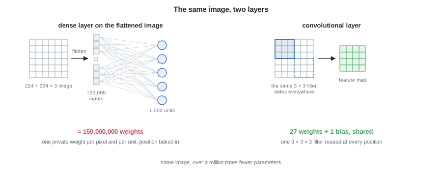 |
||||||
| 16 | ||||||||
| 17 | *The dense layer flattens the image and pays one private weight per pixel and per unit, about $150$ million in this example. The convolutional filter carries $27$ weights and one bias, and is simply reused at every position.* |
|||||||
| 18 | ||||||||
| 19 | The payoff in numbers, this time on a smaller $32 \times 32 \times 3$ input with a layer of $16$ filters (filter banks and channels are made precise in section 5.4, only the counting matters here): |
|||||||
| 20 | ||||||||
| 21 | | Layer | Weights | Biases | Total parameters | |
|||||||
| 22 | | --- | --- | --- | --- | |
|||||||
| 23 | | Convolution ($3\times3$, $16$ filters) | $3 \cdot 3 \cdot 3 \cdot 16 = 432$ | $16$ | $448$ | |
|||||||
| 24 | | Equivalent dense layer | $(32\cdot32\cdot3)\cdot(32\cdot32\cdot16) \approx 5.0\times10^{10}$ | $16{,}384$ | $\approx 5.0\times10^{10}$ | |
|||||||
| 25 | ||||||||
| 26 | A few hundred parameters against about fifty billion, and the convolution generalizes better, because the same feature detector is reused everywhere rather than relearned per position. |
|||||||
| 27 | ||||||||
|
28 | *Remark:* recall the notation from the Introduction. A layer $l$ computes $z^{[l]} = W^{[l]} a^{[l-1]} + b^{[l]}$ and $a^{[l]} = g^{[l]}(z^{[l]})$, with explicit bias $b^{[l]}$. A convolution is just a structured $W^{[l]}$ whose entries are tied together and mostly zero, so the same layer equation still holds. |
||||||
| 29 | ||||||||
|
30 | ## 5.2 The 2D convolution |
||||||
|
31 | |||||||
|
32 | ### 5.2.1 Cross-correlation |
||||||
|
33 | |||||||
| 34 | Let $I$ be a 2D input (one channel of an image) and $K$ a kernel of size $k \times k$. The operation used in deep learning slides $K$ over $I$ and takes, at each position $(i, j)$, the sum of elementwise products between the kernel and the patch it covers: |
|||||||
| 35 | ||||||||
| 36 | $$\boxed{ (I * K)_{i,j} = \sum_{m}\sum_{n} I_{i+m,\, j+n}\, K_{m,n} }$$ |
|||||||
| 37 | ||||||||
| 38 | Each output value is one dot product between the kernel and a local window of the input, so a small $3 \times 3$ kernel looks at nine pixels regardless of image size. |
|||||||
| 39 | ||||||||
|
40 | 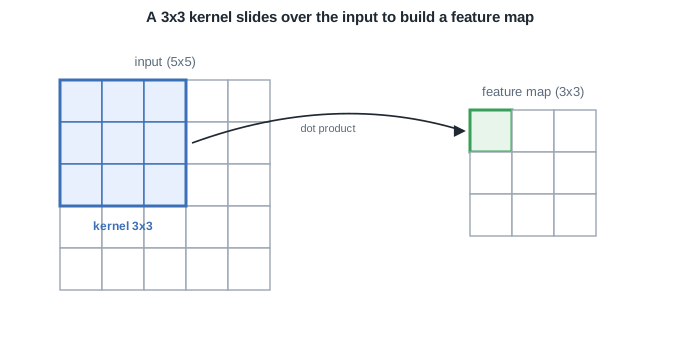 |
||||||
|
41 | |||||||
| 42 | *A convolution slides a small kernel across the input, and each position produces one cell of the output feature map.* |
|||||||
| 43 | ||||||||
| 44 | *Remark:* this is technically cross-correlation. The mathematical convolution flips the kernel first, but deep learning libraries do not flip and still call it convolution, because the learned kernel simply absorbs the flip. We follow that convention throughout. |
|||||||
| 45 | ||||||||
|
46 | ### 5.2.2 The layer output |
||||||
|
47 | |||||||
| 48 | A convolutional layer applies this operation, adds the explicit bias $b$, and passes the result through the activation $g$: |
|||||||
| 49 | ||||||||
| 50 | $$\boxed{ a^{[l]}_{i,j} = g\!\left( (a^{[l-1]} * K)_{i,j} + b \right) }$$ |
|||||||
| 51 | ||||||||
| 52 | The bias is a single scalar shared across every position of the output, exactly one more instance of parameter sharing. |
|||||||
| 53 | ||||||||
|
54 | ## 5.3 Stride, padding, and output size |
||||||
|
55 | |||||||
| 56 | Two hyperparameters control how the kernel sweeps the input. |
|||||||
| 57 | ||||||||
| 58 | - **Stride** $s$: the step in pixels between successive kernel positions. A larger stride skips positions and shrinks the output. |
|||||||
| 59 | - **Padding** $p$: a border of $p$ zeros added around the input. It lets the kernel reach the edges and controls the output size. |
|||||||
| 60 | ||||||||
| 61 | For a 1D input of size $n$ (the same formula applies per axis for 2D), the output size is: |
|||||||
| 62 | ||||||||
| 63 | $$\boxed{ o = \left\lfloor \frac{n + 2p - k}{s} \right\rfloor + 1 }$$ |
|||||||
| 64 | ||||||||
| 65 | *Remark:* two common choices have names. "Valid" padding uses $p = 0$, so the output shrinks by $k - 1$ at stride $1$. "Same" padding picks $p$ so that $o = n$ at stride $1$, which for an odd kernel means $p = (k - 1)/2$. |
|||||||
| 66 | ||||||||
| 67 | For example, with $n = 32$, $k = 5$, $p = 0$, $s = 1$ the output is $\lfloor (32 - 5)/1 \rfloor + 1 = 28$. Adding $p = 2$ ("same") gives $\lfloor (32 + 4 - 5)/1 \rfloor + 1 = 32$. |
|||||||
| 68 | ||||||||
|
69 | 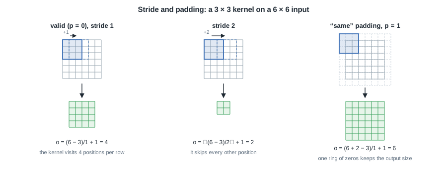 |
||||||
| 70 | ||||||||
| 71 | *The same $3 \times 3$ kernel on a $6 \times 6$ input, three ways. Stride $1$ visits four positions per row, stride $2$ skips every other one, and one ring of zero padding ($p = 1$) lets the kernel cover the border so the output keeps the input size.* |
|||||||
| 72 | ||||||||
| 73 | ## 5.4 Channels and feature maps |
|||||||
|
74 | |||||||
| 75 | Real images have channels (three for RGB), and a kernel spans all of them. A filter for an input with $C_\text{in}$ channels has shape $k \times k \times C_\text{in}$, and its convolution sums over spatial positions and channels to produce one 2D output, called a **feature map**. |
|||||||
| 76 | ||||||||
| 77 | To detect many patterns a layer stacks $C_\text{out}$ such filters, so the layer has $C_\text{out}$ feature maps and its output is a volume of shape $o \times o \times C_\text{out}$. Each feature map responds to one learned pattern (an edge orientation, a colour blob, later a texture) at every position. |
|||||||
| 78 | ||||||||
| 79 | $$\boxed{ W^{[l]} \in \mathbb{R}^{\,k \times k \times C_\text{in} \times C_\text{out}}, \qquad b^{[l]} \in \mathbb{R}^{\,C_\text{out}} }$$ |
|||||||
| 80 | ||||||||
| 81 | *Remark:* the output channel count $C_\text{out}$ of one layer becomes the input channel count $C_\text{in}$ of the next, so depth grows as spatial size shrinks. There is one bias per output channel, which is why $b^{[l]}$ has $C_\text{out}$ entries. |
|||||||
| 82 | ||||||||
|
83 | ## 5.5 Pooling |
||||||
|
84 | |||||||
| 85 | Pooling downsamples a feature map by summarising each small window with a single number, using a fixed rule and no learned weights. The two common rules are the maximum and the average over each $k \times k$ window: |
|||||||
| 86 | ||||||||
| 87 | $$\boxed{ \text{max}: \max_{m,n} a_{i+m,\, j+n} \qquad \text{avg}: \frac{1}{k^2}\sum_{m,n} a_{i+m,\, j+n} }$$ |
|||||||
| 88 | ||||||||
| 89 | Pooling with stride $s = k$ (non-overlapping windows) shrinks each spatial dimension by a factor of $k$, which cuts computation for later layers. It also grants small **translation invariance**: a max over a window returns the same value if the strong response shifts within that window. |
|||||||
| 90 | ||||||||
|
91 | 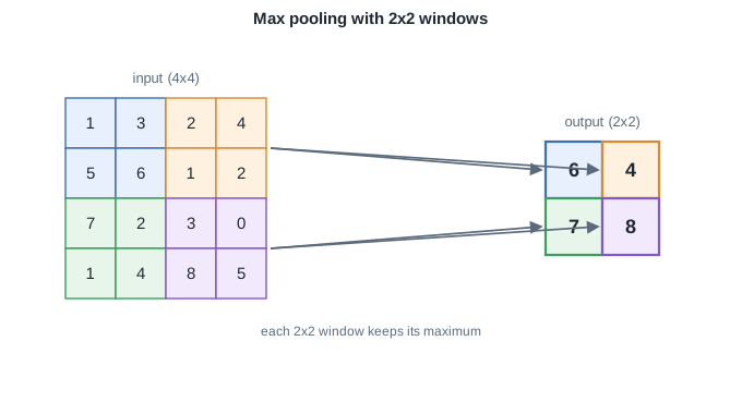 |
||||||
|
92 | |||||||
| 93 | *Max pooling downsamples each region to its largest value, shrinking the feature map and adding small translation invariance.* |
|||||||
| 94 | ||||||||
| 95 | *Remark:* pooling has no parameters and reduces resolution, which is why modern architectures often replace it with strided convolutions instead. Convolution is equivariant to translation (the response moves with the input), whereas pooling adds a little invariance (the response ignores small moves). |
|||||||
| 96 | ||||||||
|
97 | ## 5.6 A convolutional stage |
||||||
|
98 | |||||||
| 99 | A typical stage chains convolution, activation, and pooling, turning the raw image into a stack of feature maps that later stages refine. |
|||||||
| 100 | ||||||||
|
101 | 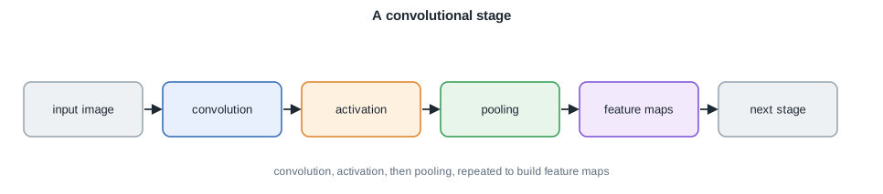 |
||||||
|
102 | |||||||
| 103 | *A convolutional stage: convolution, activation, then pooling, repeated to build feature maps.* |
|||||||
| 104 | ||||||||
| 105 | *Remark:* stacking such stages makes the receptive field (the input region that influences one output value) grow with depth, so early layers see edges and deep layers see whole objects, all built from the same local operation. |
|||||||
| 106 | ||||||||
|
107 | ## 5.7 From layers to architectures |
||||||
|
108 | |||||||
| 109 | The landmark convolutional networks all share one shape: a stack of convolution and pooling stages that extracts features, then a small fully connected head that classifies them. |
|||||||
| 110 | ||||||||
|
111 | 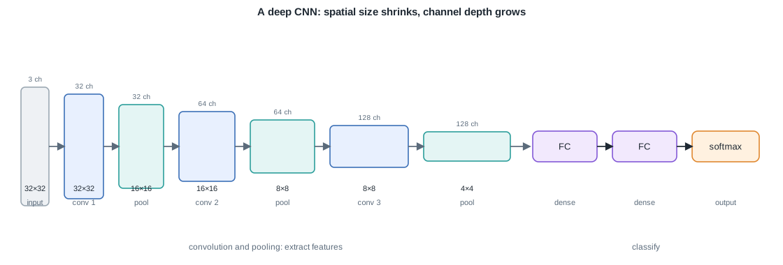 |
||||||
|
112 | |||||||
| 113 | *A deep CNN progressively reduces spatial size while increasing channel depth, then flattens into fully connected layers.* |
|||||||
| 114 | ||||||||
| 115 | Each generation contributed one idea to the same question, how to stack more layers without the training signal decaying: |
|||||||
| 116 | ||||||||
| 117 | - **LeNet**, the original, alternates a handful of convolution and pooling stages for digit recognition. |
|||||||
| 118 | - **AlexNet** scaled that skeleton to large images and GPUs, made trainable by ReLU activations and dropout. |
|||||||
| 119 | - **VGG** made every convolution $3 \times 3$ and got its depth by stacking: two $3 \times 3$ layers see the same region as one $5 \times 5$ with fewer parameters ($18c^2$ against $25c^2$) and one more nonlinearity. |
|||||||
| 120 | - **Inception** runs branches of several filter sizes in parallel and concatenates them, kept affordable by $1 \times 1$ convolutions, per-position channel maps that squeeze a thick feature map down before the expensive filters. |
|||||||
|
121 | - **ResNet** lets each block learn a correction around an identity skip connection: the skip gives the gradient a backward route that never shrinks, the direct remedy to the [vanishing gradient](/en/Deep%20Learning/02%20Activation%20functions) of lesson 2, and networks of hundreds of layers train reliably. |
||||||
|
122 | |||||||
| 123 | | Architecture | Approx. depth | Key idea | |
|||||||
| 124 | | --- | --- | --- | |
|||||||
| 125 | | LeNet | 5 to 7 layers | conv and pool stack | |
|||||||
| 126 | | AlexNet | 8 layers | ReLU and dropout at scale | |
|||||||
| 127 | | VGG | 16 to 19 layers | stacks of $3 \times 3$ convolutions | |
|||||||
| 128 | | Inception | 22 layers | parallel branches, $1 \times 1$ bottleneck | |
|||||||
| 129 | | ResNet | 50 to 152 layers | residual skip connections | |
|||||||
| 130 | ||||||||
| 131 | *Remark:* the trend is monotonic in depth, and each jump was unlocked by a specific fix: better activations, smaller filters, channel bottlenecks, and finally skip connections. |
|||||||
| 132 | ||||||||
| 133 | *These deep stacks learn feature maps whose deeper activations behave as reusable representations, the entry point of the next module on embeddings and representation learning.* |
|||||||
|
134 | |||||||
| 135 | --- |
|||||||
|
136 | Next: [Embeddings and representation learning](/en/Deep%20Learning/06%20Embeddings%20and%20representation%20learning) · [Course overview](/en/Deep%20Learning) |
||||||