Commit 36084c

2026-07-02 14:39:19 lugonthier: Add new content and images for Linear Models, Regularization, SVMs, and Decision Trees - Added images for linear regression, logistic regression, and perceptron. - Introduced a new section on Regularization and High-Dimensional Inference with detailed explanations and images. - Added content on Support Vector Machines, including definitions, loss functions, and kernel methods. - Created a new section on Decision Trees and Ensemble Methods, covering CART, bagging, random forests, and boosting. - Included relevant images to illustrate concepts in Decision Trees and Ensemble Methods.

en.md ..
@@ 1,9 1,10 @@
	# ML & MLOps Courses
-	Two courses on machine learning and putting it into production. Use the flags in the top bar to
-	change language.
+	Three courses on machine learning, deep learning, and putting models into production. Use the flags
+	in the top bar to change language.
	## Courses
	- [Machine Learning](/en/Machine%20Learning): foundations of ML, from data to models.
+	- [Deep Learning](/en/Deep%20Learning): neural networks from the perceptron to transformers.
	- [MLOps](/en/MLOps): taking ML systems to production and keeping them healthy.
/dev/null .. en/Deep Learning.md
@@ 0,0 1,28 @@
+	# Deep Learning
+
+	Neural networks from the single perceptron to modern transformers: how depth, the right activations, and gradient-based training let a model learn its own features instead of hand-crafted ones.
+
+	**Prerequisites:** the [Machine Learning](/en/Machine%20Learning) course (especially the perceptron in [Linear models](/en/Machine%20Learning/04%20Linear%20models)), basic Python, calculus, and linear algebra.
+
+	## Syllabus
+
+	1. [Introduction](/en/Deep%20Learning/01%20Introduction)
+	2. [Multilayer perceptron](/en/Deep%20Learning/02%20Multilayer%20perceptron)
+	3. [Activation functions](/en/Deep%20Learning/03%20Activation%20functions)
+	4. [Loss functions and output layers](/en/Deep%20Learning/04%20Loss%20functions%20and%20output%20layers)
+	5. [Backpropagation](/en/Deep%20Learning/05%20Backpropagation)
+	6. [Optimization](/en/Deep%20Learning/06%20Optimization)
+	7. [Initialization and vanishing gradients](/en/Deep%20Learning/07%20Initialization%20and%20vanishing%20gradients)
+	8. [Normalization](/en/Deep%20Learning/08%20Normalization)
+	9. [Regularization and dropout](/en/Deep%20Learning/09%20Regularization%20and%20dropout)
+	10. [Convolutional networks](/en/Deep%20Learning/10%20Convolutional%20networks)
+	11. [CNN architectures](/en/Deep%20Learning/11%20CNN%20architectures)
+	12. [Embeddings and representation learning](/en/Deep%20Learning/12%20Embeddings%20and%20representation%20learning)
+	13. [Recurrent networks](/en/Deep%20Learning/13%20Recurrent%20networks)
+	14. [LSTM and GRU](/en/Deep%20Learning/14%20LSTM%20and%20GRU)
+	15. [Attention](/en/Deep%20Learning/15%20Attention)
+	16. [Transformers](/en/Deep%20Learning/16%20Transformers)
+	17. [Deep learning in practice](/en/Deep%20Learning/17%20Deep%20learning%20in%20practice)
+
+	---
+	[Machine Learning](/en/Machine%20Learning) · [MLOps](/en/MLOps) · [Home](/en)
/dev/null .. en/Deep Learning/01 Introduction.md
@@ 0,0 1,103 @@
+	# 1. Introduction
+
+	This course continues directly from the Machine Learning course, which closed the [Linear models](/en/Machine%20Learning/04%20Linear%20models) part with a key remark: a perceptron is a single unit, and stacked into layers it becomes a neural network. This lesson makes that bridge explicit. It recalls what one unit can do, shows the concrete task (XOR) where a single unit fails, and fixes the notation used throughout the rest of the course.
+
+	**Objectives**
+	- Recall the perceptron as a single unit with a step activation and a linear boundary.
+	- See why one unit cannot solve XOR, motivating hidden layers.
+	- Understand what "deep" means and why hidden layers learn features.
+	- Adopt the explicit-bias, per-layer notation used across this course.
+	- Read a network as a composition of layer maps from input to prediction.
+
+	## 1.1 The perceptron, recalled
+
+	The perceptron from the Machine Learning course is a single computational unit. It scores an input with a linear combination of its features and passes that score through a hard threshold. With parameters $\theta$ and the step activation $g$, its hypothesis is:
+
+	$$\boxed{ h(x) = g(\theta^T x), \quad g(z) = \begin{cases} 1 & \text{if } z \ge 0 \\ 0 & \text{otherwise} \end{cases} }$$
+
+	The equation $\theta^T x = 0$ is a hyperplane, so the perceptron splits the input space with a single flat boundary. Points on one side are labelled $1$, points on the other are labelled $0$.
+
+	*Remark:* the boundary is linear because the score $\theta^T x$ is linear in $x$. The threshold only chooses a side, it does not bend the boundary.
+
+	## 1.2 Why one unit is not enough
+
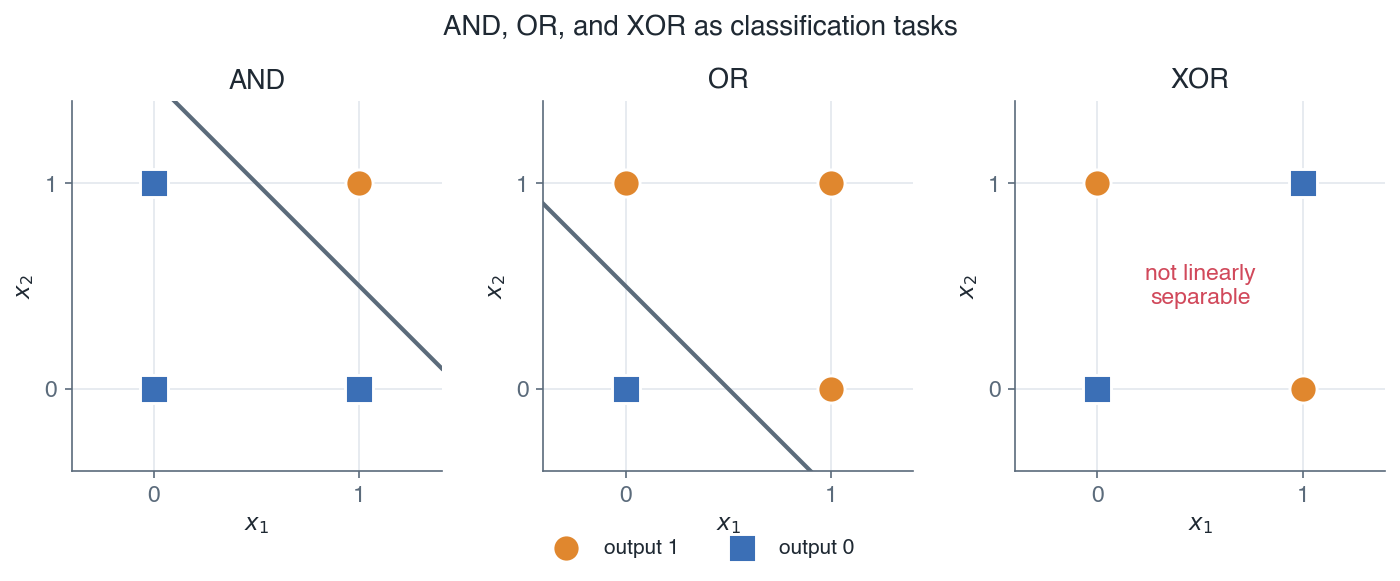
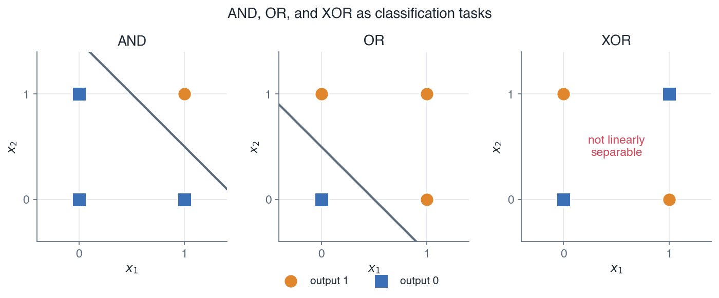
+	A single linear boundary can only solve problems whose classes are **linearly separable**, that is, separable by one straight cut. Many simple problems are, but not all. The classic counterexample is the exclusive-or (XOR) function of two binary inputs.
+
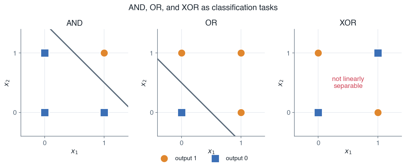
+	The truth tables below compare AND, OR, and XOR:
+
+	| $x_1$ | $x_2$ | AND | OR | XOR |
+	| --- | --- | --- | --- | --- |
+	| 0 | 0 | 0 | 0 | 0 |
+	| 0 | 1 | 0 | 1 | 1 |
+	| 1 | 0 | 0 | 1 | 1 |
+	| 1 | 1 | 1 | 1 | 0 |
+
+	
+
+	*AND and OR are separable by a single straight line, but XOR is not, which is why one unit cannot solve it.*
+
+	For AND and OR the two output classes can be separated by a single line, so a perceptron solves them. For XOR the positive points $(0,1)$ and $(1,0)$ sit on one diagonal and the negative points $(0,0)$ and $(1,1)$ sit on the other. No single straight line can separate them.
+
+	*Remark:* XOR is not a special curiosity. It shows that some patterns are inherently nonlinear, so any model built from one linear boundary is fundamentally limited. The fix is to combine several units.
+
+	If we place a layer of units between the input and the output, the first units can carve the space with several boundaries and a later unit can combine their outputs. Two lines can isolate the XOR pattern where one cannot. That intermediate layer is a **hidden layer**, and it is what turns a single unit into a network.
+
+	## 1.3 From units to networks
+
+	Stacking units into layers, and layers into a pipeline, gives a **neural network**. A network is **deep** when it has more than one hidden layer between the input and the output. Each layer applies a linear map followed by a nonlinear activation, and the layers are composed so the output of one feeds the input of the next.
+
+	The payoff is **representation learning**. In classical machine learning we hand-craft features, then feed them to a linear model. In a deep network the hidden layers learn their own features from raw input: early layers capture simple patterns and later layers combine them into more abstract ones. We specify the architecture and the objective, and the network discovers the intermediate representations by training.
+
+	*Remark:* stacking linear maps alone would collapse back to a single linear map, so the nonlinear activation $g$ between layers is essential. Without it, no depth would add expressive power. Activation functions are covered in the next lessons.
+
+	## 1.4 Notation for this course
+
+	The Machine Learning course folded the bias into the score with the intercept convention $x_0 = 1$, so a single dot product $\theta^T x$ carried the constant term. This course keeps the bias **explicit** and uses a separate weight matrix per layer. This is the seam between the two courses: from here on, no augmented input and no folded bias.
+
+	### 1.4.1 A single unit
+
+	With explicit bias, one unit has a weight vector $w$ and a scalar bias $b$. Its activation is:
+
+	$$\boxed{ a = g(w^T x + b) }$$
+
+	The score $w^T x + b$ is the same affine function as before, only now the bias $b$ is written out instead of hidden inside $\theta$.
+
+	### 1.4.2 A layer and a network
+
+	Group the units of layer $l$ into a weight matrix $W^{[l]}$ and a bias vector $b^{[l]}$. The layer computes a pre-activation $z^{[l]}$, then an activation $a^{[l]}$:
+
+	$$\boxed{ z^{[l]} = W^{[l]} a^{[l-1]} + b^{[l]}, \quad a^{[l]} = g^{[l]}(z^{[l]}) }$$
+
+	The input feeds the first layer as $a^{[0]} = x$, and for an $L$-layer network the prediction is the last activation:
+
+	$$\boxed{ a^{[0]} = x, \quad \hat{y} = a^{[L]} }$$
+
+	So the network is a composition of layer maps: $x = a^{[0]} \mapsto a^{[1]} \mapsto \cdots \mapsto a^{[L]} = \hat{y}$.
+
+	### 1.4.3 Symbol table
+
+	| Symbol | Meaning | Shape |
+	| --- | --- | --- |
+	| $L$ | number of layers | scalar |
+	| $n_l$ | number of units in layer $l$ | scalar |
+	| $W^{[l]}$ | weight matrix of layer $l$ | $n_l \times n_{l-1}$ |
+	| $b^{[l]}$ | bias vector of layer $l$ | $n_l$ |
+	| $z^{[l]}$ | pre-activation of layer $l$ | $n_l$ |
+	| $a^{[l]}$ | activation of layer $l$ | $n_l$ |
+	| $g^{[l]}$ | activation function of layer $l$ | applied elementwise |
+	| $\hat{y}$ | prediction, equal to $a^{[L]}$ | $n_L$ |
+
+	*Remark:* the activation $g^{[l]}$ acts componentwise, so an elementwise product later on is written with the Hadamard symbol $\odot$. The superscript in brackets, $[l]$, indexes the layer, not an exponent.
+
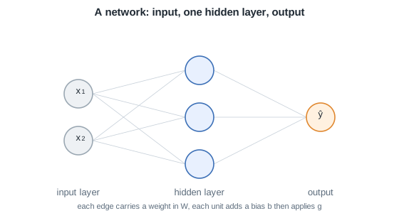
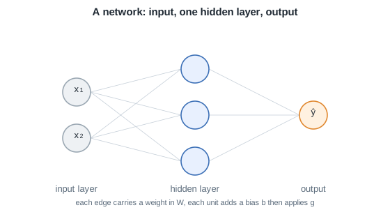
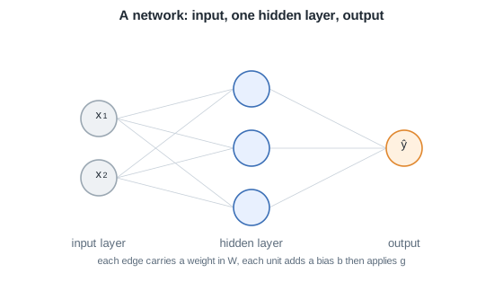
+	The following diagram shows the smallest useful network: an input layer, one hidden layer, and an output layer.
+
+	
+
+	*A neural network: an input layer, one hidden layer, and an output. Each edge carries a weight and each unit adds a bias then applies an activation g.*
+
+	Each arrow carries a weight from $W^{[l]}$, and every hidden and output unit adds its bias from $b^{[l]}$ before applying its activation. This two-unit hidden layer is exactly what lets the network solve XOR, the task that defeated a single unit.
+
+	*The next lesson formalizes this picture as the multilayer perceptron, writing the full forward pass layer by layer and choosing the activation functions.*
+
+	---
+	Next: [Multilayer perceptron](/en/Deep%20Learning/02%20Multilayer%20perceptron) · [Course overview](/en/Deep%20Learning)
/dev/null .. en/Deep Learning/01 Introduction/network-single-hidden.svg
@@ 0,0 1,1 @@
+	<svg xmlns="http://www.w3.org/2000/svg" viewBox="0 0 560 314" width="560" height="314" font-family="Helvetica, Arial, sans-serif"><defs><marker id="arrow" viewBox="0 0 10 10" refX="8.5" refY="5" markerWidth="7" markerHeight="7" orient="auto-start-reverse"><path d="M0 0L10 5L0 10z" fill="#1f2933"/></marker><marker id="arrowmuted" viewBox="0 0 10 10" refX="8.5" refY="5" markerWidth="7" markerHeight="7" orient="auto-start-reverse"><path d="M0 0L10 5L0 10z" fill="#5b6b7b"/></marker></defs><rect width="560" height="314" fill="#ffffff"/><text x="280.0" y="22.0" font-family="Helvetica, Arial, sans-serif" font-size="15" font-weight="600" fill="#1f2933" text-anchor="middle">A network: input, one hidden layer, output</text><line x1="130.0" y1="132.0" x2="260.0" y2="99.0" stroke="#c7d0d9" stroke-width="0.8"/><line x1="130.0" y1="132.0" x2="260.0" y2="165.0" stroke="#c7d0d9" stroke-width="0.8"/><line x1="130.0" y1="132.0" x2="260.0" y2="231.0" stroke="#c7d0d9" stroke-width="0.8"/><line x1="130.0" y1="198.0" x2="260.0" y2="99.0" stroke="#c7d0d9" stroke-width="0.8"/><line x1="130.0" y1="198.0" x2="260.0" y2="165.0" stroke="#c7d0d9" stroke-width="0.8"/><line x1="130.0" y1="198.0" x2="260.0" y2="231.0" stroke="#c7d0d9" stroke-width="0.8"/><line x1="300.0" y1="99.0" x2="430.0" y2="165.0" stroke="#c7d0d9" stroke-width="0.8"/><line x1="300.0" y1="165.0" x2="430.0" y2="165.0" stroke="#c7d0d9" stroke-width="0.8"/><line x1="300.0" y1="231.0" x2="430.0" y2="165.0" stroke="#c7d0d9" stroke-width="0.8"/><circle cx="110.0" cy="132.0" r="20.0" fill="#eef1f4" stroke="#9aa7b2" stroke-width="1.6"/><circle cx="110.0" cy="198.0" r="20.0" fill="#eef1f4" stroke="#9aa7b2" stroke-width="1.6"/><circle cx="280.0" cy="99.0" r="20.0" fill="#e8f0fe" stroke="#3b6fb6" stroke-width="1.6"/><circle cx="280.0" cy="165.0" r="20.0" fill="#e8f0fe" stroke="#3b6fb6" stroke-width="1.6"/><circle cx="280.0" cy="231.0" r="20.0" fill="#e8f0fe" stroke="#3b6fb6" stroke-width="1.6"/><circle cx="450.0" cy="165.0" r="20.0" fill="#fff1e0" stroke="#e0872e" stroke-width="1.6"/><text x="110.0" y="275.0" font-family="Helvetica, Arial, sans-serif" font-size="13" fill="#5b6b7b" text-anchor="middle">input layer</text><text x="280.0" y="275.0" font-family="Helvetica, Arial, sans-serif" font-size="13" fill="#5b6b7b" text-anchor="middle">hidden layer</text><text x="450.0" y="275.0" font-family="Helvetica, Arial, sans-serif" font-size="13" fill="#5b6b7b" text-anchor="middle">output</text><text x="110.0" y="132.0" font-family="Helvetica, Arial, sans-serif" font-size="13" fill="#1f2933" text-anchor="middle">x<tspan baseline-shift="sub" font-size="9px">1</tspan></text><text x="110.0" y="198.0" font-family="Helvetica, Arial, sans-serif" font-size="13" fill="#1f2933" text-anchor="middle">x<tspan baseline-shift="sub" font-size="9px">2</tspan></text><text x="450.0" y="165.0" font-family="Helvetica, Arial, sans-serif" font-size="13" fill="#1f2933" text-anchor="middle">ŷ</text><text x="280.0" y="294.0" font-family="Helvetica, Arial, sans-serif" font-size="11" fill="#5b6b7b" text-anchor="middle">each edge carries a weight in W, each unit adds a bias b then applies g</text></svg>
\	No newline at end of file
/dev/null .. en/Deep Learning/01 Introduction/xor-problem.png
/dev/null .. en/Deep Learning/02 Multilayer perceptron.md
@@ 0,0 1,100 @@
+	# 2. Multilayer perceptron
+
+	A perceptron is one unit, $a = g(w^T x + b)$. Stack many units that read the same input and you get a layer, stack layers and you get a multilayer perceptron (MLP). This module builds the MLP from units, writes forward propagation for one example and for a mini-batch, tracks the shapes and the parameter count, and states the universal approximation theorem.
+
+	**Objectives**
+	- Build a layer as a stack of perceptron-like units reading a shared input.
+	- Write forward propagation for one example with explicit per-layer weights and bias.
+	- Vectorize the forward pass over a mini-batch with broadcast bias.
+	- Track the shape of every $W^{[l]}$ and $b^{[l]}$ and count the parameters.
+	- State the universal approximation theorem and contrast width against depth.
+
+	## 2.1 From a unit to a layer
+
+	### 2.1.1 A single unit
+
+	A unit takes an input vector $x \in \mathbb{R}^{n_0}$, forms a weighted sum with a weight vector $w$ and a bias scalar $b$, then applies a nonlinear activation $g$:
+
+	$$\boxed{ a = g\left(w^T x + b\right) }$$
+
+	This is the perceptron of the previous course, except the hard step is now a smooth activation such as the sigmoid or ReLU. The activation is named here and defined fully in the [next lesson](/en/Deep%20Learning/03%20Activation%20functions).
+
+	### 2.1.2 A layer of units
+
+	Now place $n_1$ units side by side, all reading the same input $x$. Unit $i$ has its own weight vector $w_i$ and bias $b_i$, producing $a_i = g(w_i^T x + b_i)$. Collect the weight vectors as the rows of a matrix $W^{[1]}$ and the biases into a vector $b^{[1]}$:
+
+	$$\boxed{ W^{[1]} = \begin{bmatrix} w_1^{T} \\ \vdots \\ w_{n_1}^{T} \end{bmatrix}, \quad b^{[1]} = \begin{bmatrix} b_1 \\ \vdots \\ b_{n_1} \end{bmatrix} }$$
+
+	The whole layer then computes a pre-activation vector and an activation vector in one matrix expression, $z^{[1]} = W^{[1]} x + b^{[1]}$ and $a^{[1]} = g^{[1]}(z^{[1]})$, where $g^{[1]}$ is applied elementwise.
+
+	*Remark:* the rows of $W^{[1]}$ are exactly the individual unit weight vectors, so a layer is just many units packed into one matrix. Bias stays explicit here: unlike the Machine Learning course, which folded the intercept into $\theta$ via the augmented input $x_0 = 1$, this course keeps $b^{[l]}$ as its own vector.
+
+	## 2.2 Forward propagation
+
+	Stacking $L$ such layers gives the MLP. Layer $l$ reads the activation of the layer below, $a^{[l-1]}$, and produces $a^{[l]}$. The input is $a^{[0]} = x$ and the prediction is the output of the last layer.
+
+	### 2.2.1 One example
+
+	For $l = 1, \dots, L$:
+
+	$$\boxed{ a^{[0]} = x, \quad z^{[l]} = W^{[l]} a^{[l-1]} + b^{[l]}, \quad a^{[l]} = g^{[l]}\!\left(z^{[l]}\right), \quad \hat{y} = a^{[L]} }$$
+
+	Each layer may use its own activation $g^{[l]}$: hidden layers typically use ReLU, while the output layer uses sigmoid or softmax for classification and the identity for regression.
+
+	*Remark:* the composition $\hat{y} = g^{[L]}(W^{[L]} g^{[L-1]}(\cdots g^{[1]}(W^{[1]} x + b^{[1]}) \cdots) + b^{[L]})$ is what makes the network expressive. Without the nonlinear $g^{[l]}$ the whole stack would collapse to a single linear map $W x + b$.
+
+	### 2.2.2 Vectorized over a mini-batch
+
+	Training runs on batches, not single examples. Place $m$ examples as the columns of a matrix, so $A^{[0]} = X \in \mathbb{R}^{n_0 \times m}$, and the forward pass becomes a matrix product with the bias broadcast across all columns:
+
+	$$\boxed{ Z^{[l]} = W^{[l]} A^{[l-1]} + b^{[l]}, \quad A^{[l]} = g^{[l]}\!\left(Z^{[l]}\right) }$$
+
+	Here $Z^{[l]}$ and $A^{[l]}$ have shape $n_l \times m$, one column per example. The bias $b^{[l]} \in \mathbb{R}^{n_l}$ is added to every column, an operation known as broadcasting.
+
+	*Remark:* the only change from the single-example form is that the vector $a^{[l-1]}$ becomes the matrix $A^{[l-1]}$. Processing a batch as one matrix multiply is what lets a GPU run the pass efficiently.
+
+	## 2.3 Shapes and parameter count
+
+	The shapes follow from one rule: to compute $z^{[l]} = W^{[l]} a^{[l-1]} + b^{[l]}$, the matrix $W^{[l]}$ must map an $n_{l-1}$-vector to an $n_l$-vector.
+
+	$$\boxed{ W^{[l]} \in \mathbb{R}^{n_l \times n_{l-1}}, \quad b^{[l]} \in \mathbb{R}^{n_l} }$$
+
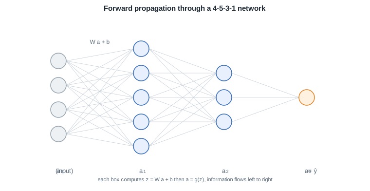
+	Layer $l$ therefore holds $n_l \, n_{l-1}$ weights plus $n_l$ biases. Consider a small network with $n_0 = 4$ inputs, two hidden layers of $5$ and $3$ units, and a single output unit.
+
+	| Layer $l$ | $W^{[l]}$ shape | $b^{[l]}$ shape | Parameters |
+	| --- | --- | --- | --- |
+	| 1 | $5 \times 4$ | $5$ | $25$ |
+	| 2 | $3 \times 5$ | $3$ | $18$ |
+	| 3 | $1 \times 3$ | $1$ | $4$ |
+	| Total | | | $47$ |
+
+	*Remark:* the input layer holds no parameters, it is just the data $a^{[0]} = x$. When counting layers we count the layers that carry weights, so this network has $L = 3$.
+
+	## 2.4 A multi-layer network
+
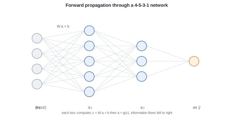
+	The diagram below shows the same $4$-$5$-$3$-$1$ network as a flow of activations. Each arrow group is a full weight matrix, and each box applies its activation to the pre-activation.
+
+	
+
+	*A multilayer perceptron: each layer computes z = W a + b then a = g(z), composing input a0 into the prediction aL.*
+
+	Information flows strictly left to right during the forward pass, which is why this is a feedforward network. Nothing loops back. The reverse direction, used to compute gradients, is the subject of a later lesson.
+
+	## 2.5 Universal approximation
+
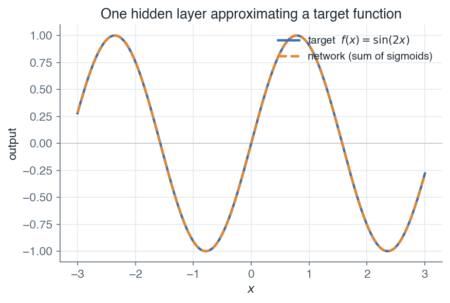
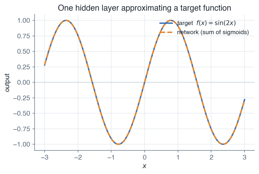
+	How expressive is an MLP? The universal approximation theorem gives a strong answer. Let $f$ be any continuous function on a compact set $K \subset \mathbb{R}^{n_0}$, and let $\varepsilon > 0$. Then there exists a network with a single hidden layer of finite width, using a suitable nonlinear activation, whose output $F$ satisfies:
+
+	$$\boxed{ \sup_{x \in K} \left| F(x) - f(x) \right| < \varepsilon }$$
+
+	In words, one hidden layer with enough units can approximate any continuous function on a bounded region to any desired accuracy $\varepsilon$. This is an existence result, not a recipe: it promises that such weights exist, but says nothing about how many units are needed or how to find them.
+
+	*Remark:* the catch is width. Matching a target to accuracy $\varepsilon$ with one hidden layer can demand an enormous number of units, growing fast as $\varepsilon$ shrinks. Depth is usually far more parameter-efficient: stacking several narrow layers can represent functions that a single layer would need exponentially many units to match. This efficiency of depth over width is the practical reason the field is called deep learning.
+
+	
+
+	*A network with one hidden layer approximates a target function by summing many simple activated units.*
+
+	*The network is only defined once the activations $g^{[l]}$ are fixed. The next lesson defines them, sigmoid, tanh, ReLU and its variants, and explains how each shapes learning.*
+
+	---
+	Next: [Activation functions](/en/Deep%20Learning/03%20Activation%20functions) · [Course overview](/en/Deep%20Learning)
/dev/null .. en/Deep Learning/02 Multilayer perceptron/mlp-forward.svg
@@ 0,0 1,1 @@
+	<svg xmlns="http://www.w3.org/2000/svg" viewBox="0 0 760 392" width="760" height="392" font-family="Helvetica, Arial, sans-serif"><defs><marker id="arrow" viewBox="0 0 10 10" refX="8.5" refY="5" markerWidth="7" markerHeight="7" orient="auto-start-reverse"><path d="M0 0L10 5L0 10z" fill="#1f2933"/></marker><marker id="arrowmuted" viewBox="0 0 10 10" refX="8.5" refY="5" markerWidth="7" markerHeight="7" orient="auto-start-reverse"><path d="M0 0L10 5L0 10z" fill="#5b6b7b"/></marker></defs><rect width="760" height="392" fill="#ffffff"/><text x="380.0" y="22.0" font-family="Helvetica, Arial, sans-serif" font-size="15" font-weight="600" fill="#1f2933" text-anchor="middle">Forward propagation through a 4-5-3-1 network</text><line x1="136.0" y1="125.0" x2="274.0" y2="100.0" stroke="#c7d0d9" stroke-width="0.8"/><line x1="136.0" y1="125.0" x2="274.0" y2="150.0" stroke="#c7d0d9" stroke-width="0.8"/><line x1="136.0" y1="125.0" x2="274.0" y2="200.0" stroke="#c7d0d9" stroke-width="0.8"/><line x1="136.0" y1="125.0" x2="274.0" y2="250.0" stroke="#c7d0d9" stroke-width="0.8"/><line x1="136.0" y1="125.0" x2="274.0" y2="300.0" stroke="#c7d0d9" stroke-width="0.8"/><line x1="136.0" y1="175.0" x2="274.0" y2="100.0" stroke="#c7d0d9" stroke-width="0.8"/><line x1="136.0" y1="175.0" x2="274.0" y2="150.0" stroke="#c7d0d9" stroke-width="0.8"/><line x1="136.0" y1="175.0" x2="274.0" y2="200.0" stroke="#c7d0d9" stroke-width="0.8"/><line x1="136.0" y1="175.0" x2="274.0" y2="250.0" stroke="#c7d0d9" stroke-width="0.8"/><line x1="136.0" y1="175.0" x2="274.0" y2="300.0" stroke="#c7d0d9" stroke-width="0.8"/><line x1="136.0" y1="225.0" x2="274.0" y2="100.0" stroke="#c7d0d9" stroke-width="0.8"/><line x1="136.0" y1="225.0" x2="274.0" y2="150.0" stroke="#c7d0d9" stroke-width="0.8"/><line x1="136.0" y1="225.0" x2="274.0" y2="200.0" stroke="#c7d0d9" stroke-width="0.8"/><line x1="136.0" y1="225.0" x2="274.0" y2="250.0" stroke="#c7d0d9" stroke-width="0.8"/><line x1="136.0" y1="225.0" x2="274.0" y2="300.0" stroke="#c7d0d9" stroke-width="0.8"/><line x1="136.0" y1="275.0" x2="274.0" y2="100.0" stroke="#c7d0d9" stroke-width="0.8"/><line x1="136.0" y1="275.0" x2="274.0" y2="150.0" stroke="#c7d0d9" stroke-width="0.8"/><line x1="136.0" y1="275.0" x2="274.0" y2="200.0" stroke="#c7d0d9" stroke-width="0.8"/><line x1="136.0" y1="275.0" x2="274.0" y2="250.0" stroke="#c7d0d9" stroke-width="0.8"/><line x1="136.0" y1="275.0" x2="274.0" y2="300.0" stroke="#c7d0d9" stroke-width="0.8"/><line x1="306.0" y1="100.0" x2="444.0" y2="150.0" stroke="#c7d0d9" stroke-width="0.8"/><line x1="306.0" y1="100.0" x2="444.0" y2="200.0" stroke="#c7d0d9" stroke-width="0.8"/><line x1="306.0" y1="100.0" x2="444.0" y2="250.0" stroke="#c7d0d9" stroke-width="0.8"/><line x1="306.0" y1="150.0" x2="444.0" y2="150.0" stroke="#c7d0d9" stroke-width="0.8"/><line x1="306.0" y1="150.0" x2="444.0" y2="200.0" stroke="#c7d0d9" stroke-width="0.8"/><line x1="306.0" y1="150.0" x2="444.0" y2="250.0" stroke="#c7d0d9" stroke-width="0.8"/><line x1="306.0" y1="200.0" x2="444.0" y2="150.0" stroke="#c7d0d9" stroke-width="0.8"/><line x1="306.0" y1="200.0" x2="444.0" y2="200.0" stroke="#c7d0d9" stroke-width="0.8"/><line x1="306.0" y1="200.0" x2="444.0" y2="250.0" stroke="#c7d0d9" stroke-width="0.8"/><line x1="306.0" y1="250.0" x2="444.0" y2="150.0" stroke="#c7d0d9" stroke-width="0.8"/><line x1="306.0" y1="250.0" x2="444.0" y2="200.0" stroke="#c7d0d9" stroke-width="0.8"/><line x1="306.0" y1="250.0" x2="444.0" y2="250.0" stroke="#c7d0d9" stroke-width="0.8"/><line x1="306.0" y1="300.0" x2="444.0" y2="150.0" stroke="#c7d0d9" stroke-width="0.8"/><line x1="306.0" y1="300.0" x2="444.0" y2="200.0" stroke="#c7d0d9" stroke-width="0.8"/><line x1="306.0" y1="300.0" x2="444.0" y2="250.0" stroke="#c7d0d9" stroke-width="0.8"/><line x1="476.0" y1="150.0" x2="614.0" y2="200.0" stroke="#c7d0d9" stroke-width="0.8"/><line x1="476.0" y1="200.0" x2="614.0" y2="200.0" stroke="#c7d0d9" stroke-width="0.8"/><line x1="476.0" y1="250.0" x2="614.0" y2="200.0" stroke="#c7d0d9" stroke-width="0.8"/><circle cx="120.0" cy="125.0" r="16.0" fill="#eef1f4" stroke="#9aa7b2" stroke-width="1.6"/><circle cx="120.0" cy="175.0" r="16.0" fill="#eef1f4" stroke="#9aa7b2" stroke-width="1.6"/><circle cx="120.0" cy="225.0" r="16.0" fill="#eef1f4" stroke="#9aa7b2" stroke-width="1.6"/><circle cx="120.0" cy="275.0" r="16.0" fill="#eef1f4" stroke="#9aa7b2" stroke-width="1.6"/><circle cx="290.0" cy="100.0" r="16.0" fill="#e8f0fe" stroke="#3b6fb6" stroke-width="1.6"/><circle cx="290.0" cy="150.0" r="16.0" fill="#e8f0fe" stroke="#3b6fb6" stroke-width="1.6"/><circle cx="290.0" cy="200.0" r="16.0" fill="#e8f0fe" stroke="#3b6fb6" stroke-width="1.6"/><circle cx="290.0" cy="250.0" r="16.0" fill="#e8f0fe" stroke="#3b6fb6" stroke-width="1.6"/><circle cx="290.0" cy="300.0" r="16.0" fill="#e8f0fe" stroke="#3b6fb6" stroke-width="1.6"/><circle cx="460.0" cy="150.0" r="16.0" fill="#e8f0fe" stroke="#3b6fb6" stroke-width="1.6"/><circle cx="460.0" cy="200.0" r="16.0" fill="#e8f0fe" stroke="#3b6fb6" stroke-width="1.6"/><circle cx="460.0" cy="250.0" r="16.0" fill="#e8f0fe" stroke="#3b6fb6" stroke-width="1.6"/><circle cx="630.0" cy="200.0" r="16.0" fill="#fff1e0" stroke="#e0872e" stroke-width="1.6"/><text x="120.0" y="355.0" font-family="Helvetica, Arial, sans-serif" font-size="13" fill="#5b6b7b" text-anchor="middle">a<tspan baseline-shift="sub" font-size="9px">0</tspan> (input)</text><text x="290.0" y="355.0" font-family="Helvetica, Arial, sans-serif" font-size="13" fill="#5b6b7b" text-anchor="middle">a<tspan baseline-shift="sub" font-size="9px">1</tspan></text><text x="460.0" y="355.0" font-family="Helvetica, Arial, sans-serif" font-size="13" fill="#5b6b7b" text-anchor="middle">a<tspan baseline-shift="sub" font-size="9px">2</tspan></text><text x="630.0" y="355.0" font-family="Helvetica, Arial, sans-serif" font-size="13" fill="#5b6b7b" text-anchor="middle">a<tspan baseline-shift="sub" font-size="9px">3</tspan> = ŷ</text><text x="205.0" y="90.0" font-family="Helvetica, Arial, sans-serif" font-size="12" fill="#5b6b7b" text-anchor="middle">W a + b</text><text x="380.0" y="372.0" font-family="Helvetica, Arial, sans-serif" font-size="11" fill="#5b6b7b" text-anchor="middle">each box computes z = W a + b then a = g(z), information flows left to right</text></svg>
\	No newline at end of file
/dev/null .. en/Deep Learning/02 Multilayer perceptron/universal-approximation.png
/dev/null .. en/Deep Learning/03 Activation functions.md
@@ 0,0 1,103 @@
+	# 3. Activation functions
+
+	Each layer computes a pre-activation $z^{[l]} = W^{[l]} a^{[l-1]} + b^{[l]}$ and then an activation $a^{[l]} = g^{[l]}(z^{[l]})$. The choice of the nonlinearity $g^{[l]}$ is what makes depth worthwhile. This lesson explains why a nonlinear $g$ is required, surveys the sigmoid, tanh, and ReLU families, introduces the softmax used at the output, and gives practical guidance on which activation to pick.
+
+	**Objectives**
+	- Show that a stack of purely linear layers collapses to a single linear map.
+	- Define the sigmoid and tanh, derive their derivatives, and explain saturation.
+	- Survey the ReLU family (ReLU, leaky ReLU, PReLU, ELU, GELU) and the dead-unit problem.
+	- Define the softmax and place it at the output rather than in hidden layers.
+	- Give a short rule of thumb for choosing an activation per layer.
+
+	## 3.1 Why nonlinearity is required
+
+	Suppose every activation were the identity, $g^{[l]}(z) = z$. Then each layer is just $a^{[l]} = W^{[l]} a^{[l-1]} + b^{[l]}$, and composing two of them gives $W^{[2]}(W^{[1]} x + b^{[1]}) + b^{[2]} = (W^{[2]} W^{[1]}) x + (W^{[2]} b^{[1]} + b^{[2]})$. That is again of the form $W x + b$. By induction the whole $L$-layer network reduces to a single affine map:
+
+	$$\boxed{ g^{[l]} = \text{identity} \;\Rightarrow\; \hat{y} = W' x + b' }$$
+
+	with $W' = W^{[L]} \cdots W^{[1]}$ and $b'$ the accumulated bias. No matter how many linear layers are stacked, the model can only fit a linear function, so the extra depth buys nothing. A nonlinear $g$ between layers is exactly what breaks this collapse and lets the network represent curved decision boundaries and nonlinear regressions.
+
+	*Remark:* the bias is kept explicit here as $b^{[l]}$, unlike the Machine Learning course where the intercept was folded into $\theta^T x$ via the augmented input $x_0 = 1$. In this Deep Learning course each layer has its own weight matrix $W^{[l]}$ and its own bias vector $b^{[l]}$.
+
+	## 3.2 Sigmoid and tanh
+
+	
+
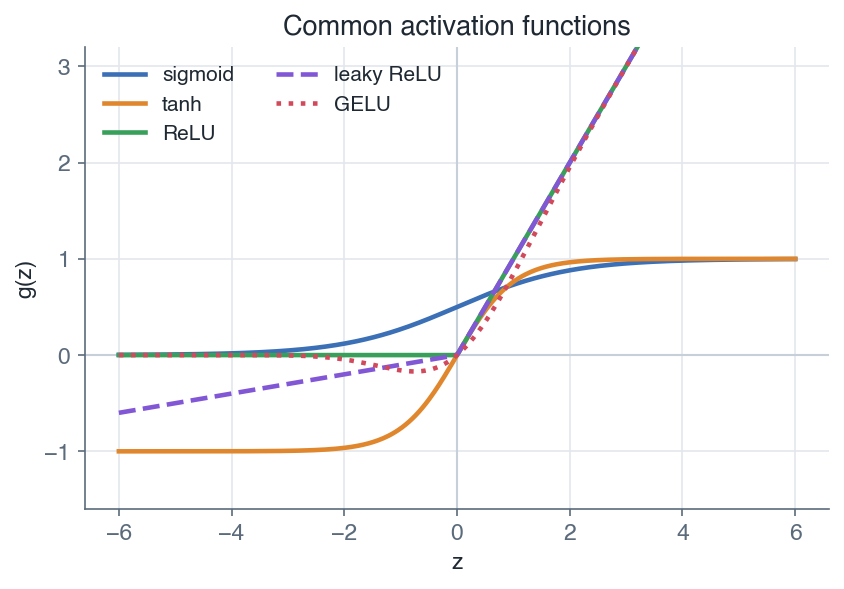
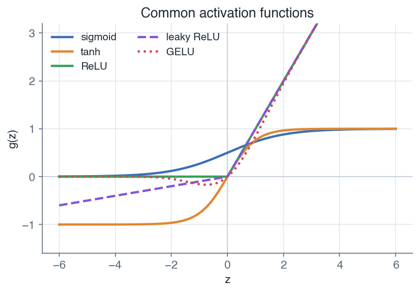
+	*Common activation functions: the bounded sigmoid and tanh saturate in their tails, while ReLU and its variants stay linear for positive inputs.*
+
+	### 3.2.1 Sigmoid
+
+	The sigmoid squashes any real pre-activation into the open interval $(0, 1)$:
+
+	$$\boxed{ \sigma(z) = \frac{1}{1 + e^{-z}} \in (0, 1) }$$
+
+	Its derivative has the convenient closed form below, which reuses the forward value $\sigma(z)$ already computed:
+
+	$$\boxed{ \sigma'(z) = \sigma(z)\left(1 - \sigma(z)\right) }$$
+
+	### 3.2.2 Tanh
+
+	The hyperbolic tangent is a rescaled sigmoid centred at zero, with output in $(-1, 1)$. Its derivative is likewise expressible from the forward value:
+
+	$$\boxed{ \tanh'(z) = 1 - \tanh(z)^2 }$$
+
+	*Remark:* $\tanh$ is zero-centred while $\sigma$ is not, so $\tanh$ often trains a little better as a hidden activation. The two are related by $\tanh(z) = 2\sigma(2z) - 1$.
+
+	### 3.2.3 Saturation
+
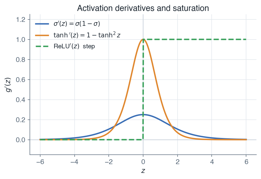
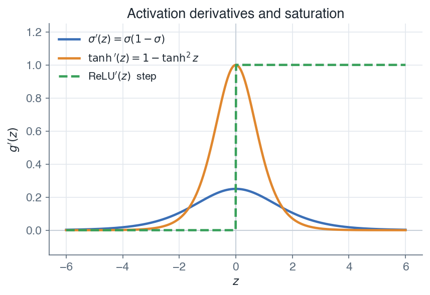
+	Both curves flatten in their tails. For large $|z|$ the output is close to a constant ($0$ or $1$ for $\sigma$, $\pm 1$ for $\tanh$), so the derivative is close to zero: $\sigma'(z) \to 0$ and $\tanh'(z) \to 0$. A unit sitting in that flat region is said to saturate, and it passes almost no gradient backward. When many such factors multiply through a deep stack the gradient shrinks toward zero, the vanishing-gradient problem revisited in [Initialization and vanishing gradients](/en/Deep%20Learning/07%20Initialization%20and%20vanishing%20gradients).
+
+	
+
+	*Activation derivatives: sigmoid and tanh gradients vanish in the tails, whereas the ReLU gradient is 1 wherever the unit is active.*
+
+	## 3.3 The ReLU family
+
+	The rectified linear unit keeps the positive part of its input and zeroes the rest:
+
+	$$\boxed{ \text{ReLU}(z) = \max(0, z) }$$
+
+	Its derivative is $1$ for $z > 0$ and $0$ for $z < 0$ (undefined at $z = 0$, taken to be $0$ or $1$ by convention). ReLU does not saturate on the positive side, so it keeps a healthy gradient flowing there, which is a large part of why it became the default hidden activation. The cost is the dead-unit problem: if a unit's pre-activation is always negative across the data, its gradient is always zero and it stops learning entirely. The variants below trade a little simplicity to soften that failure or to smooth the kink at the origin.
+
+	| name | formula | derivative | dies / saturates? |
+	| --- | --- | --- | --- |
+	| ReLU | $\max(0, z)$ | $1$ if $z>0$ else $0$ | can die (zero gradient for $z<0$) |
+	| Leaky ReLU | $\max(\alpha z, z)$, $\alpha \approx 0.01$ | $1$ if $z>0$ else $\alpha$ | rarely dies (small negative slope) |
+	| PReLU | $\max(\alpha z, z)$, $\alpha$ learned | $1$ if $z>0$ else $\alpha$ | rarely dies ($\alpha$ trained per channel) |
+	| ELU | $z$ if $z>0$ else $\alpha(e^z - 1)$ | $1$ if $z>0$ else $\alpha e^z$ | saturates gently for $z\to-\infty$ |
+	| GELU | $z\,\Phi(z)$, $\Phi$ the normal CDF | smooth, near $1$ for large $z$ | smooth, no hard death |
+
+	*Remark:* leaky ReLU and PReLU add a small slope $\alpha$ on the negative side so a unit is never fully switched off. GELU weights the input by the probability $\Phi(z)$ that a standard normal is below $z$, giving a smooth curve that behaves like ReLU for large $|z|$. It is the standard choice inside Transformers.
+
+	## 3.4 Softmax for multiclass outputs
+
+	For a classification with $K$ classes the final layer outputs a vector $z \in \mathbb{R}^K$ of scores, and the softmax turns it into a probability distribution over the classes:
+
+	$$\boxed{ \text{softmax}(z)_k = \frac{e^{z_k}}{\sum_{j=1}^{K} e^{z_j}} }$$
+
+	Each component lies in $(0, 1)$ and the components sum to $1$, so $\text{softmax}(z)_k$ reads as the predicted probability of class $k$. The largest score becomes the most likely class.
+
+	*Remark:* softmax belongs at the output layer, not in a hidden layer. It couples every unit through the shared denominator (a normalization across the whole vector), which is exactly what a probability output needs but is not a useful per-unit hidden nonlinearity. For a single output ($K = 1$ vs its complement) softmax reduces to the sigmoid. The pairing of softmax with its loss is the subject of [Loss functions and output layers](/en/Deep%20Learning/04%20Loss%20functions%20and%20output%20layers).
+
+	## 3.5 Choosing an activation
+
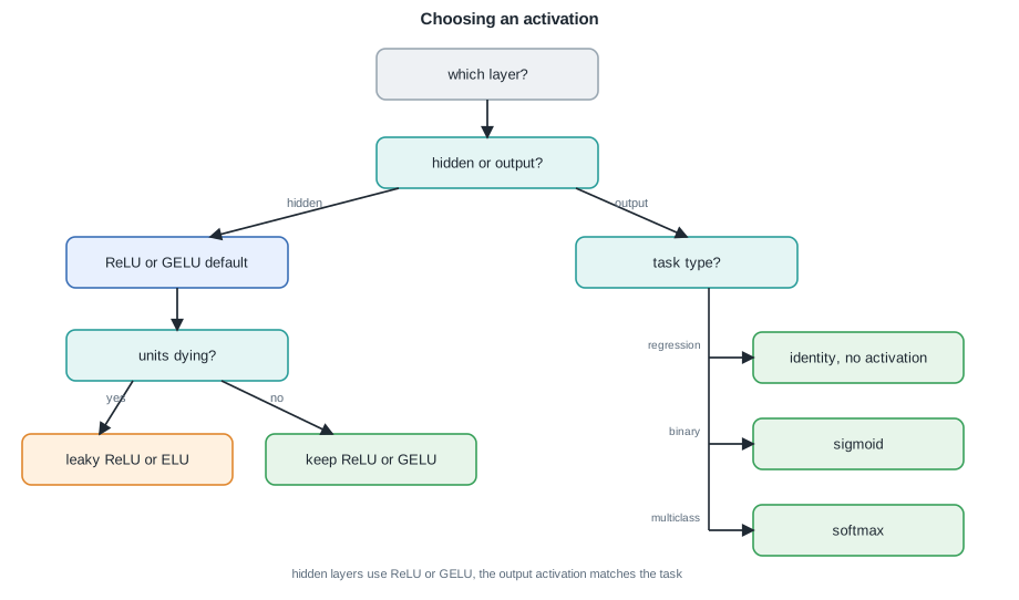
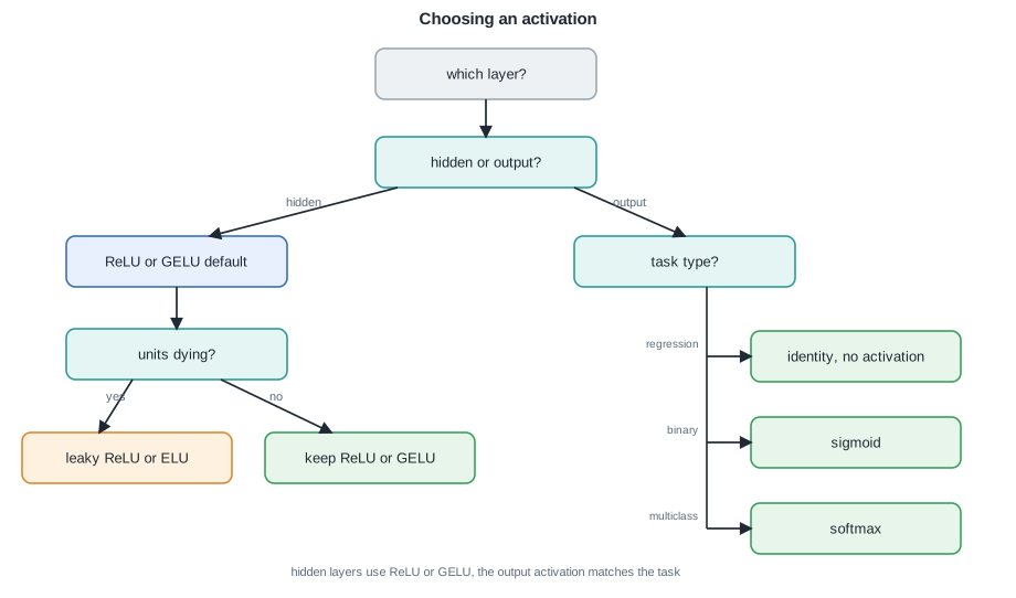
+	A useful default: use ReLU or GELU in the hidden layers, and choose the output activation from the task. The diagram and table below summarize the decision.
+
+	
+
+	*Choosing an activation: ReLU or GELU for hidden layers, and an output activation matched to the task.*
+
+	| layer / task | recommended activation | reason |
+	| --- | --- | --- |
+	| hidden (default) | ReLU or GELU | no positive-side saturation, cheap, trains fast |
+	| hidden (dead units) | leaky ReLU or ELU | keeps a nonzero gradient for $z < 0$ |
+	| output, regression | identity (none) | prediction is an unbounded real value |
+	| output, binary | sigmoid | maps score to a probability in $(0, 1)$ |
+	| output, multiclass | softmax | maps scores to a distribution over classes |
+
+	*Remark:* sigmoid and tanh are now rarely used as hidden activations in deep feed-forward networks precisely because of the saturation in Section 3.2.3. They survive at the output (sigmoid) and inside gated recurrent units, where their bounded range is the point.
+
+	*With the per-layer nonlinearities fixed, the next lesson pairs the output activation with a matching loss so the network has something to minimize.*
+
+	---
+	Next: [Loss functions and output layers](/en/Deep%20Learning/04%20Loss%20functions%20and%20output%20layers) · [Course overview](/en/Deep%20Learning)
/dev/null .. en/Deep Learning/03 Activation functions/activation-choice.svg
@@ 0,0 1,1 @@
+	<svg xmlns="http://www.w3.org/2000/svg" viewBox="0 0 920 542" width="920" height="542" font-family="Helvetica, Arial, sans-serif"><defs><marker id="arrow" viewBox="0 0 10 10" refX="8.5" refY="5" markerWidth="7" markerHeight="7" orient="auto-start-reverse"><path d="M0 0L10 5L0 10z" fill="#1f2933"/></marker><marker id="arrowmuted" viewBox="0 0 10 10" refX="8.5" refY="5" markerWidth="7" markerHeight="7" orient="auto-start-reverse"><path d="M0 0L10 5L0 10z" fill="#5b6b7b"/></marker></defs><rect width="920" height="542" fill="#ffffff"/><text x="460.0" y="22.0" font-family="Helvetica, Arial, sans-serif" font-size="15" font-weight="600" fill="#1f2933" text-anchor="middle">Choosing an activation</text><rect x="340.0" y="44.0" width="200.0" height="46.0" rx="8" fill="#eef1f4" stroke="#9aa7b2" stroke-width="1.6"/><text x="440.0" y="71.4" font-family="Helvetica, Arial, sans-serif" font-size="13" fill="#1f2933" text-anchor="middle">which layer?</text><rect x="340.0" y="124.0" width="200.0" height="46.0" rx="8" fill="#e4f5f4" stroke="#2a9d9a" stroke-width="1.6"/><text x="440.0" y="151.4" font-family="Helvetica, Arial, sans-serif" font-size="13" fill="#1f2933" text-anchor="middle">hidden or output?</text><line x1="440.0" y1="90.0" x2="440.0" y2="124.0" stroke="#1f2933" stroke-width="1.7" marker-end="url(#arrow)"/><rect x="60.0" y="214.0" width="200.0" height="46.0" rx="8" fill="#e8f0fe" stroke="#3b6fb6" stroke-width="1.6"/><text x="160.0" y="241.4" font-family="Helvetica, Arial, sans-serif" font-size="13" fill="#1f2933" text-anchor="middle">ReLU or GELU default</text><line x1="360.0" y1="170.0" x2="190.0" y2="214.0" stroke="#1f2933" stroke-width="1.7" marker-end="url(#arrow)"/><text x="275.0" y="187.0" font-family="Helvetica, Arial, sans-serif" font-size="11" fill="#5b6b7b" text-anchor="middle">hidden</text><rect x="60.0" y="298.0" width="200.0" height="46.0" rx="8" fill="#e4f5f4" stroke="#2a9d9a" stroke-width="1.6"/><text x="160.0" y="325.4" font-family="Helvetica, Arial, sans-serif" font-size="13" fill="#1f2933" text-anchor="middle">units dying?</text><line x1="160.0" y1="260.0" x2="160.0" y2="298.0" stroke="#1f2933" stroke-width="1.7" marker-end="url(#arrow)"/><rect x="20.0" y="392.0" width="190.0" height="46.0" rx="8" fill="#fff1e0" stroke="#e0872e" stroke-width="1.6"/><text x="115.0" y="419.4" font-family="Helvetica, Arial, sans-serif" font-size="13" fill="#1f2933" text-anchor="middle">leaky ReLU or ELU</text><line x1="120.0" y1="344.0" x2="90.0" y2="392.0" stroke="#1f2933" stroke-width="1.7" marker-end="url(#arrow)"/><text x="105.0" y="363.0" font-family="Helvetica, Arial, sans-serif" font-size="11" fill="#5b6b7b" text-anchor="middle">yes</text><rect x="240.0" y="392.0" width="190.0" height="46.0" rx="8" fill="#e7f5ea" stroke="#38a05a" stroke-width="1.6"/><text x="335.0" y="419.4" font-family="Helvetica, Arial, sans-serif" font-size="13" fill="#1f2933" text-anchor="middle">keep ReLU or GELU</text><line x1="200.0" y1="344.0" x2="300.0" y2="392.0" stroke="#1f2933" stroke-width="1.7" marker-end="url(#arrow)"/><text x="250.0" y="363.0" font-family="Helvetica, Arial, sans-serif" font-size="11" fill="#5b6b7b" text-anchor="middle">no</text><rect x="520.0" y="214.0" width="200.0" height="46.0" rx="8" fill="#e4f5f4" stroke="#2a9d9a" stroke-width="1.6"/><text x="620.0" y="241.4" font-family="Helvetica, Arial, sans-serif" font-size="13" fill="#1f2933" text-anchor="middle">task type?</text><line x1="520.0" y1="170.0" x2="620.0" y2="214.0" stroke="#1f2933" stroke-width="1.7" marker-end="url(#arrow)"/><text x="570.0" y="187.0" font-family="Helvetica, Arial, sans-serif" font-size="11" fill="#5b6b7b" text-anchor="middle">output</text><line x1="640.0" y1="260.0" x2="640.0" y2="479.0" stroke="#1f2933" stroke-width="1.6"/><rect x="680.0" y="300.0" width="190.0" height="46.0" rx="8" fill="#e7f5ea" stroke="#38a05a" stroke-width="1.6"/><text x="775.0" y="327.4" font-family="Helvetica, Arial, sans-serif" font-size="13" fill="#1f2933" text-anchor="middle">identity, no activation</text><line x1="640.0" y1="323.0" x2="680.0" y2="323.0" stroke="#1f2933" stroke-width="1.7" marker-end="url(#arrow)"/><text x="632.0" y="315.0" font-family="Helvetica, Arial, sans-serif" font-size="10" fill="#5b6b7b" text-anchor="end">regression</text><rect x="680.0" y="378.0" width="190.0" height="46.0" rx="8" fill="#e7f5ea" stroke="#38a05a" stroke-width="1.6"/><text x="775.0" y="405.4" font-family="Helvetica, Arial, sans-serif" font-size="13" fill="#1f2933" text-anchor="middle">sigmoid</text><line x1="640.0" y1="401.0" x2="680.0" y2="401.0" stroke="#1f2933" stroke-width="1.7" marker-end="url(#arrow)"/><text x="632.0" y="393.0" font-family="Helvetica, Arial, sans-serif" font-size="10" fill="#5b6b7b" text-anchor="end">binary</text><rect x="680.0" y="456.0" width="190.0" height="46.0" rx="8" fill="#e7f5ea" stroke="#38a05a" stroke-width="1.6"/><text x="775.0" y="483.4" font-family="Helvetica, Arial, sans-serif" font-size="13" fill="#1f2933" text-anchor="middle">softmax</text><line x1="640.0" y1="479.0" x2="680.0" y2="479.0" stroke="#1f2933" stroke-width="1.7" marker-end="url(#arrow)"/><text x="632.0" y="471.0" font-family="Helvetica, Arial, sans-serif" font-size="10" fill="#5b6b7b" text-anchor="end">multiclass</text><text x="440.0" y="522.0" font-family="Helvetica, Arial, sans-serif" font-size="11" fill="#5b6b7b" text-anchor="middle">hidden layers use ReLU or GELU, the output activation matches the task</text></svg>
\	No newline at end of file
/dev/null .. en/Deep Learning/03 Activation functions/activation-derivatives.png
/dev/null .. en/Deep Learning/03 Activation functions/activation-functions.png
/dev/null .. en/Deep Learning/04 Loss functions and output layers.md
@@ 0,0 1,92 @@
+	# 4. Loss functions and output layers
+
+	Before a network can learn it needs a target to descend toward. The output layer turns the last activation $a^{[L]}$ into a prediction, and the loss measures how far that prediction is from the true label. This module fixes both choices per task, because backpropagation in the next module differentiates a concrete loss. The output activation and the loss are not picked independently: matching them to the task shape is what makes the training signal clean.
+
+	**Objectives**
+	- Go from a per-example loss $L$ to the cost $J$ averaged over the batch.
+	- Choose a linear output with mean squared error for regression.
+	- Choose a sigmoid output with binary cross-entropy for two-class problems.
+	- Choose a softmax output with categorical cross-entropy for multiclass problems.
+	- Derive the clean logit gradient of the softmax and cross-entropy pair.
+	- Map any task to its output activation and loss with a single lookup table.
+
+	## 4.1 From per-example loss to cost
+
+	The network predicts $\hat{y} = a^{[L]}$ from input $a^{[0]} = x$. For a single example the loss $L(\hat{y}, y)$ scores that prediction against the target $y$. Training minimizes the cost $J$, defined as the average of $L$ over the $m$ examples in the batch or dataset:
+
+	$$\boxed{ J = \frac{1}{m}\sum_{i=1}^{m} L\!\left(\hat{y}^{(i)}, y^{(i)}\right) }$$
+
+	*Remark:* the loss $L$ scores one prediction, the cost $J$ is what the optimizer actually reduces. Averaging (rather than summing) keeps the gradient scale independent of the batch size, so the learning rate does not have to be retuned when $m$ changes.
+
+	The three tasks below reuse the losses introduced in the Machine Learning course. The cross-entropy row of the loss table at [General concepts](/en/Machine%20Learning/02%20General%20concepts), labelled "Neural networks", is exactly the objective a classification network minimizes. The novelty here is pairing each loss with the output activation $g^{[L]}$ that produces $\hat{y}$.
+
+	## 4.2 Regression: linear output and mean squared error
+
+	For a continuous target $y \in \mathbb{R}^{n_L}$ the output layer uses no activation, so it is linear (the identity) and the prediction can take any real value:
+
+	$$\boxed{ \hat{y} = a^{[L]} = z^{[L]} = W^{[L]} a^{[L-1]} + b^{[L]} }$$
+
+	The per-example loss is the squared Euclidean distance between prediction and target, scaled by one half:
+
+	$$\boxed{ L(\hat{y}, y) = \tfrac{1}{2}\,\lVert \hat{y} - y \rVert^2 }$$
+
+	*Remark:* the factor $\tfrac{1}{2}$ cancels the $2$ that appears on differentiating the square, leaving the tidy residual gradient $\partial L / \partial \hat{y} = \hat{y} - y$. This is the same mean-squared-error objective used for linear regression, now sitting on top of a deep network instead of a single linear score.
+
+	## 4.3 Binary classification: sigmoid output and binary cross-entropy
+
+	For a two-class label $y \in \{0, 1\}$ the output layer has a single unit whose activation is the sigmoid, squashing the logit $z^{[L]}$ into a probability:
+
+	$$\hat{y} = a^{[L]} = \sigma\!\left(z^{[L]}\right) = \frac{1}{1 + e^{-z^{[L]}}} \in (0, 1)$$
+
+	Here $\hat{y}$ is read as $p(y = 1 \mid x)$. The matching loss is the binary cross-entropy, the negative log-likelihood of the Bernoulli label:
+
+	$$\boxed{ L(\hat{y}, y) = -\Big[\, y \log \hat{y} + (1 - y)\log(1 - \hat{y}) \,\Big] }$$
+
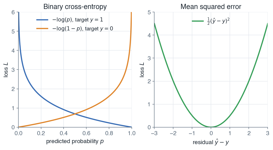
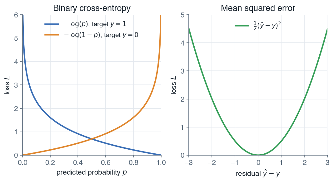
+	*Remark:* only one of the two terms is active for any given label. When $y = 1$ the loss is $-\log \hat{y}$, penalizing a small predicted probability, and when $y = 0$ it is $-\log(1 - \hat{y})$. Cross-entropy is preferred over squared error here because it keeps the gradient large when the prediction is confidently wrong, so learning does not stall.
+
+	
+
+	*Cross-entropy loss grows without bound as the predicted probability moves away from the true label.*
+
+	## 4.4 Multiclass classification: softmax output and categorical cross-entropy
+
+	For a $K$-class label the output layer has $K$ units and the softmax activation turns the logit vector $z^{[L]} \in \mathbb{R}^{K}$ into a probability distribution over the classes:
+
+	$$\boxed{ \hat{y}_k = \frac{e^{z^{[L]}_k}}{\sum_{j=1}^{K} e^{z^{[L]}_j}} }$$
+
+	The outputs are positive and sum to one, so $\hat{y}$ is a proper distribution and $\hat{y}_k = p(y = k \mid x)$. The target $y$ is one-hot: $y_k = 1$ for the true class and $0$ otherwise. The matching loss is the categorical cross-entropy:
+
+	$$\boxed{ L(\hat{y}, y) = -\sum_{k=1}^{K} y_k \log \hat{y}_k }$$
+
+	*Remark:* because $y$ is one-hot the sum collapses to a single term, $-\log \hat{y}_{k^\star}$, where $k^\star$ is the true class. The loss therefore rewards putting probability mass on the correct class and ignores how the remaining mass is split. Binary cross-entropy is the special case $K = 2$.
+
+	## 4.5 The softmax and cross-entropy gradient
+
+	The softmax output and the categorical cross-entropy loss are used together because their composition has a remarkably clean derivative at the logits $z^{[L]}$. Differentiating $L$ with respect to a single logit $z^{[L]}_k$ gives:
+
+	$$\boxed{ \frac{\partial L}{\partial z^{[L]}_k} = \hat{y}_k - y_k }$$
+
+	The gradient at the output layer is just the prediction minus the target, a plain residual with no awkward sigmoid or softmax factor left over. The same identity holds for the sigmoid and binary cross-entropy pair, which is its $K = 2$ instance. This is precisely why each activation is coupled to its matching loss rather than mixed with, say, squared error.
+
+	*Remark:* the elementwise form $\partial L / \partial z^{[L]} = \hat{y} - y$ is what seeds backpropagation. The next module starts the backward pass from this vector and then repeatedly applies the chain rule and the Hadamard product $\odot$ to push it back through the hidden layers.
+
+	## 4.6 Task to output to loss
+
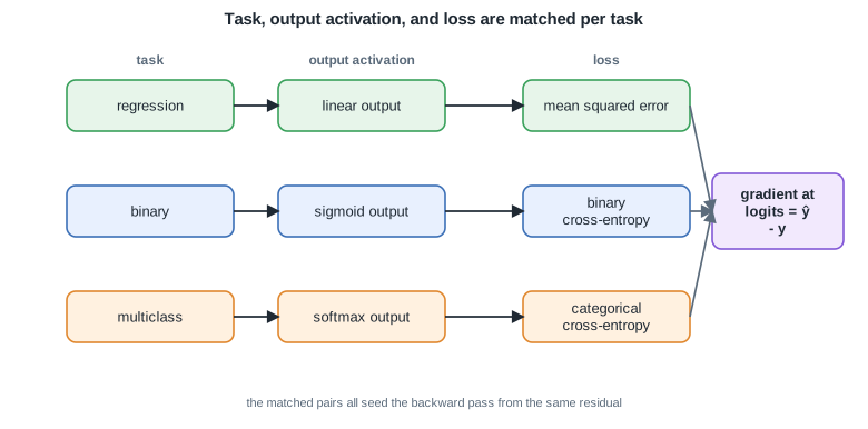
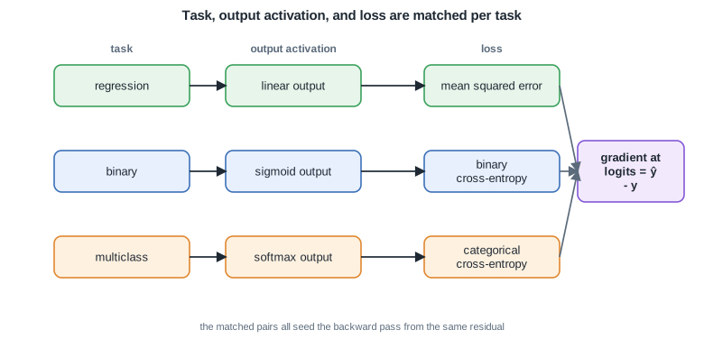
+	The three cases collapse into one lookup. Fix the task, and the output activation and loss follow.
+
+	| Task | Output activation $g^{[L]}$ | Per-example loss $L$ | Logit gradient $\partial L / \partial z^{[L]}$ |
+	| --- | --- | --- | --- |
+	| Regression | linear (identity) | mean squared error | $\hat{y} - y$ |
+	| Binary classification | sigmoid | binary cross-entropy | $\hat{y} - y$ |
+	| Multiclass classification | softmax | categorical cross-entropy | $\hat{y} - y$ |
+
+	*Remark:* the last column is identical across all three rows. Matching the output activation to its natural loss makes the network start its backward pass from the same simple residual regardless of the task.
+
+	
+
+	*The output activation and loss are chosen together per task, and the matched pairs share the clean logit gradient yhat minus y.*
+
+	*With a concrete loss chosen and its output-layer gradient in hand, the next module runs the chain rule backward through every layer: backpropagation.*
+
+	---
+	Next: [Backpropagation](/en/Deep%20Learning/05%20Backpropagation) · [Course overview](/en/Deep%20Learning)
/dev/null .. en/Deep Learning/04 Loss functions and output layers/loss-curves.png
/dev/null .. en/Deep Learning/04 Loss functions and output layers/output-loss-map.svg
@@ 0,0 1,1 @@
+	<svg xmlns="http://www.w3.org/2000/svg" viewBox="0 0 780 386" width="780" height="386" font-family="Helvetica, Arial, sans-serif"><defs><marker id="arrow" viewBox="0 0 10 10" refX="8.5" refY="5" markerWidth="7" markerHeight="7" orient="auto-start-reverse"><path d="M0 0L10 5L0 10z" fill="#1f2933"/></marker><marker id="arrowmuted" viewBox="0 0 10 10" refX="8.5" refY="5" markerWidth="7" markerHeight="7" orient="auto-start-reverse"><path d="M0 0L10 5L0 10z" fill="#5b6b7b"/></marker></defs><rect width="780" height="386" fill="#ffffff"/><text x="390.0" y="22.0" font-family="Helvetica, Arial, sans-serif" font-size="15" font-weight="600" fill="#1f2933" text-anchor="middle">Task, output activation, and loss are matched per task</text><text x="135.0" y="58.0" font-family="Helvetica, Arial, sans-serif" font-size="12" font-weight="600" fill="#5b6b7b" text-anchor="middle">task</text><text x="325.0" y="58.0" font-family="Helvetica, Arial, sans-serif" font-size="12" font-weight="600" fill="#5b6b7b" text-anchor="middle">output activation</text><text x="545.0" y="58.0" font-family="Helvetica, Arial, sans-serif" font-size="12" font-weight="600" fill="#5b6b7b" text-anchor="middle">loss</text><rect x="640.0" y="156.0" width="118.0" height="68.0" rx="8" fill="#f2e9fd" stroke="#8257d6" stroke-width="1.6"/><text x="699.0" y="179.1" font-family="Helvetica, Arial, sans-serif" font-size="13" font-weight="600" fill="#1f2933" text-anchor="middle">gradient at</text><text x="699.0" y="194.4" font-family="Helvetica, Arial, sans-serif" font-size="13" font-weight="600" fill="#1f2933" text-anchor="middle">logits = ŷ</text><text x="699.0" y="209.8" font-family="Helvetica, Arial, sans-serif" font-size="13" font-weight="600" fill="#1f2933" text-anchor="middle">- y</text><rect x="60.0" y="72.0" width="150.0" height="46.0" rx="8" fill="#e7f5ea" stroke="#38a05a" stroke-width="1.6"/><text x="135.0" y="99.4" font-family="Helvetica, Arial, sans-serif" font-size="13" fill="#1f2933" text-anchor="middle">regression</text><rect x="250.0" y="72.0" width="150.0" height="46.0" rx="8" fill="#e7f5ea" stroke="#38a05a" stroke-width="1.6"/><text x="325.0" y="99.4" font-family="Helvetica, Arial, sans-serif" font-size="13" fill="#1f2933" text-anchor="middle">linear output</text><rect x="470.0" y="72.0" width="150.0" height="46.0" rx="8" fill="#e7f5ea" stroke="#38a05a" stroke-width="1.6"/><text x="545.0" y="99.4" font-family="Helvetica, Arial, sans-serif" font-size="13" fill="#1f2933" text-anchor="middle">mean squared error</text><line x1="210.0" y1="95.0" x2="250.0" y2="95.0" stroke="#1f2933" stroke-width="1.7" marker-end="url(#arrow)"/><line x1="400.0" y1="95.0" x2="470.0" y2="95.0" stroke="#1f2933" stroke-width="1.7" marker-end="url(#arrow)"/><line x1="620.0" y1="95.0" x2="640.0" y2="190.0" stroke="#5b6b7b" stroke-width="1.7" marker-end="url(#arrowmuted)"/><rect x="60.0" y="167.0" width="150.0" height="46.0" rx="8" fill="#e8f0fe" stroke="#3b6fb6" stroke-width="1.6"/><text x="135.0" y="194.4" font-family="Helvetica, Arial, sans-serif" font-size="13" fill="#1f2933" text-anchor="middle">binary</text><rect x="250.0" y="167.0" width="150.0" height="46.0" rx="8" fill="#e8f0fe" stroke="#3b6fb6" stroke-width="1.6"/><text x="325.0" y="194.4" font-family="Helvetica, Arial, sans-serif" font-size="13" fill="#1f2933" text-anchor="middle">sigmoid output</text><rect x="470.0" y="167.0" width="150.0" height="46.0" rx="8" fill="#e8f0fe" stroke="#3b6fb6" stroke-width="1.6"/><text x="545.0" y="186.8" font-family="Helvetica, Arial, sans-serif" font-size="13" fill="#1f2933" text-anchor="middle">binary</text><text x="545.0" y="202.1" font-family="Helvetica, Arial, sans-serif" font-size="13" fill="#1f2933" text-anchor="middle">cross-entropy</text><line x1="210.0" y1="190.0" x2="250.0" y2="190.0" stroke="#1f2933" stroke-width="1.7" marker-end="url(#arrow)"/><line x1="400.0" y1="190.0" x2="470.0" y2="190.0" stroke="#1f2933" stroke-width="1.7" marker-end="url(#arrow)"/><line x1="620.0" y1="190.0" x2="640.0" y2="190.0" stroke="#5b6b7b" stroke-width="1.7" marker-end="url(#arrowmuted)"/><rect x="60.0" y="262.0" width="150.0" height="46.0" rx="8" fill="#fff1e0" stroke="#e0872e" stroke-width="1.6"/><text x="135.0" y="289.4" font-family="Helvetica, Arial, sans-serif" font-size="13" fill="#1f2933" text-anchor="middle">multiclass</text><rect x="250.0" y="262.0" width="150.0" height="46.0" rx="8" fill="#fff1e0" stroke="#e0872e" stroke-width="1.6"/><text x="325.0" y="289.4" font-family="Helvetica, Arial, sans-serif" font-size="13" fill="#1f2933" text-anchor="middle">softmax output</text><rect x="470.0" y="262.0" width="150.0" height="46.0" rx="8" fill="#fff1e0" stroke="#e0872e" stroke-width="1.6"/><text x="545.0" y="281.8" font-family="Helvetica, Arial, sans-serif" font-size="13" fill="#1f2933" text-anchor="middle">categorical</text><text x="545.0" y="297.1" font-family="Helvetica, Arial, sans-serif" font-size="13" fill="#1f2933" text-anchor="middle">cross-entropy</text><line x1="210.0" y1="285.0" x2="250.0" y2="285.0" stroke="#1f2933" stroke-width="1.7" marker-end="url(#arrow)"/><line x1="400.0" y1="285.0" x2="470.0" y2="285.0" stroke="#1f2933" stroke-width="1.7" marker-end="url(#arrow)"/><line x1="620.0" y1="285.0" x2="640.0" y2="190.0" stroke="#5b6b7b" stroke-width="1.7" marker-end="url(#arrowmuted)"/><text x="390.0" y="366.0" font-family="Helvetica, Arial, sans-serif" font-size="11" fill="#5b6b7b" text-anchor="middle">the matched pairs all seed the backward pass from the same residual</text></svg>
\	No newline at end of file
/dev/null .. en/Deep Learning/05 Backpropagation.md
@@ 0,0 1,100 @@
+	# 5. Backpropagation
+
+	Backpropagation is the algorithm that computes the gradient of the cost with respect to every parameter of a network. It is nothing more than the chain rule applied in a careful, reverse order over the computational graph, reusing the quantities cached during the forward pass. This module derives it layer by layer using the error signal $\delta^{[l]} = \partial L / \partial z^{[l]}$.
+
+	**Objectives**
+	- Read a network as a composition of functions and see why gradients flow backward by the chain rule.
+	- Define the layer error $\delta^{[l]}$ and compute the output-layer error $\delta^{[L]}$.
+	- Establish the backward recursion that carries $\delta$ from layer $L$ down to layer $1$.
+	- Turn each $\delta^{[l]}$ into the parameter gradients for $W^{[l]}$ and $b^{[l]}$.
+	- Assemble the full forward-and-backward algorithm and connect it to the parameter update.
+
+	## 5.1 The chain rule over a computational graph
+
+	A feedforward network is a composition of functions. Each layer $l$ takes the previous activation $a^{[l-1]}$ and produces a pre-activation and an activation:
+
+	$$\boxed{ z^{[l]} = W^{[l]} a^{[l-1]} + b^{[l]}, \quad a^{[l]} = g^{[l]}\!\left(z^{[l]}\right) }$$
+
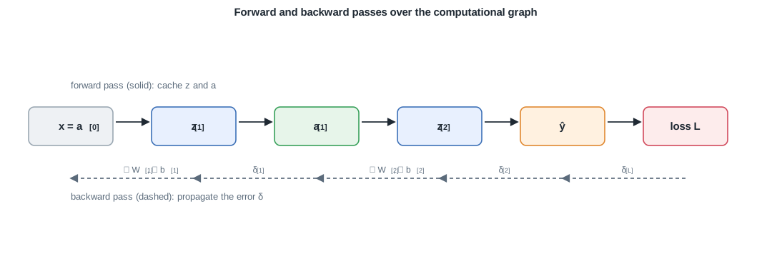
+	with $a^{[0]} = x$ and prediction $\hat{y} = a^{[L]}$. The scalar loss $L$ sits at the end of this chain. Because the cost is a composition, its derivative with respect to any intermediate quantity is a product of local derivatives, one per link in the graph. The chain rule tells us to accumulate those products.
+
+	The efficient way to do this is to walk the graph backward. A single reverse traversal computes, for every node, the derivative of the final loss with respect to that node, and each step reuses the derivative already computed for the node just downstream. This reuse is what makes backpropagation cost about the same as one forward pass, rather than one pass per parameter.
+
+	
+
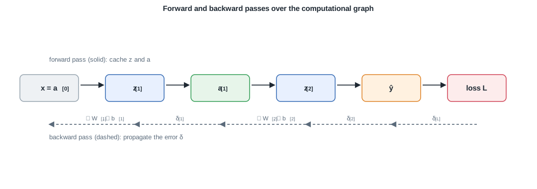
+	*Backpropagation traverses the computational graph in reverse: the forward pass (solid) caches values, the backward pass (dashed) propagates the error delta.*
+
+	*Remark:* the solid arrows are the forward pass (data flowing to the loss) and the dashed arrows are the backward pass (gradients flowing from the loss). The two passes traverse the same graph in opposite directions.
+
+	## 5.2 The layer error
+
+	The central object is the error of layer $l$, the sensitivity of the loss to the pre-activation $z^{[l]}$:
+
+	$$\boxed{ \delta^{[l]} = \frac{\partial L}{\partial z^{[l]}} \in \mathbb{R}^{n_l} }$$
+
+	Once we know $\delta^{[l]}$ at every layer, all parameter gradients follow immediately (Section 5.5). The whole algorithm reduces to computing these vectors, first at the output layer, then recursively backward.
+
+	*Remark:* placing $\delta$ at the pre-activation $z^{[l]}$ rather than at the activation $a^{[l]}$ is a deliberate choice. It makes the activation derivative $g'^{[l]}$ appear exactly once per layer and keeps the recursion clean.
+
+	## 5.3 Output-layer error
+
+	At the output layer the chain rule has two links: the loss depends on $a^{[L]} = \hat{y}$, and $a^{[L]}$ depends on $z^{[L]}$ through the activation $g^{[L]}$. Multiplying the two local derivatives elementwise gives the output error:
+
+	$$\boxed{ \delta^{[L]} = \nabla_{a^{[L]}} L \;\odot\; g'^{[L]}\!\left(z^{[L]}\right) }$$
+
+	The Hadamard product $\odot$ appears because $g^{[L]}$ acts elementwise, so component $j$ of $z^{[L]}$ influences only component $j$ of $a^{[L]}$.
+
+	### 5.3.1 The softmax and cross-entropy shortcut
+
+	For multiclass classification the natural pairing is a softmax output with the cross-entropy loss (introduced in [Loss functions and output layers](/en/Deep%20Learning/04%20Loss%20functions%20and%20output%20layers)). The two derivatives combine and cancel, leaving a strikingly simple result:
+
+	$$\boxed{ \delta^{[L]} = \hat{y} - y }$$
+
+	*Remark:* the same clean form appears for a sigmoid output with binary cross-entropy, and for a linear output with squared error. In each case the output activation is the matched inverse link of the loss, so the messy factors cancel and the error is just the residual $\hat{y} - y$.
+
+	## 5.4 The backward recursion
+
+	Given the error at layer $l+1$, we obtain the error at layer $l$. The loss depends on $z^{[l]}$ only through $z^{[l+1]} = W^{[l+1]} a^{[l]} + b^{[l]}$, and $a^{[l]} = g^{[l]}(z^{[l]})$. Propagating the sensitivity back through the weight matrix and then through the activation gives:
+
+	$$\boxed{ \delta^{[l]} = \left( \left(W^{[l+1]}\right)^{T} \delta^{[l+1]} \right) \odot g'^{[l]}\!\left(z^{[l]}\right) }$$
+
+	Two operations happen here. The transpose $\left(W^{[l+1]}\right)^{T}$ sends the downstream error back across the linear map, spreading each downstream component onto the units that fed it. The elementwise product with $g'^{[l]}(z^{[l]})$ then filters it by how sensitive each activation was at its operating point.
+
+	| Symbol | Meaning | Shape |
+	| --- | --- | --- |
+	| $\delta^{[l]}$ | error at layer $l$ | $(n_l)$ |
+	| $W^{[l+1]}$ | weights into layer $l+1$ | $(n_{l+1} \times n_l)$ |
+	| $\left(W^{[l+1]}\right)^{T}\delta^{[l+1]}$ | error pushed back to layer $l$ | $(n_l)$ |
+	| $g'^{[l]}(z^{[l]})$ | local activation slope | $(n_l)$ |
+
+	*Remark:* the forward pass uses $W^{[l+1]}$ and the backward pass uses its transpose. This is the same linear map read in reverse, which is why the backward pass has the same cost as the forward pass.
+
+	## 5.5 Parameter gradients
+
+	The error $\delta^{[l]}$ is all we need for the parameters of layer $l$. Since $z^{[l]} = W^{[l]} a^{[l-1]} + b^{[l]}$ is linear in $W^{[l]}$ and $b^{[l]}$, the last chain-rule link is easy. The weight gradient is the outer product of the layer error with the cached input activation:
+
+	$$\boxed{ \frac{\partial L}{\partial W^{[l]}} = \delta^{[l]} \left(a^{[l-1]}\right)^{T}, \qquad \frac{\partial L}{\partial b^{[l]}} = \delta^{[l]} }$$
+
+	The weight gradient has shape $(n_l \times n_{l-1})$, matching $W^{[l]}$, and the bias gradient has shape $(n_l)$, matching $b^{[l]}$. The bias gradient is exactly $\delta^{[l]}$ because $\partial z^{[l]} / \partial b^{[l]}$ is the identity.
+
+	*Remark:* the cached activation $a^{[l-1]}$ from the forward pass is reused verbatim in the weight gradient. This is the concrete payoff of caching: nothing from the forward pass is recomputed.
+
+	## 5.6 The full algorithm
+
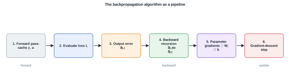
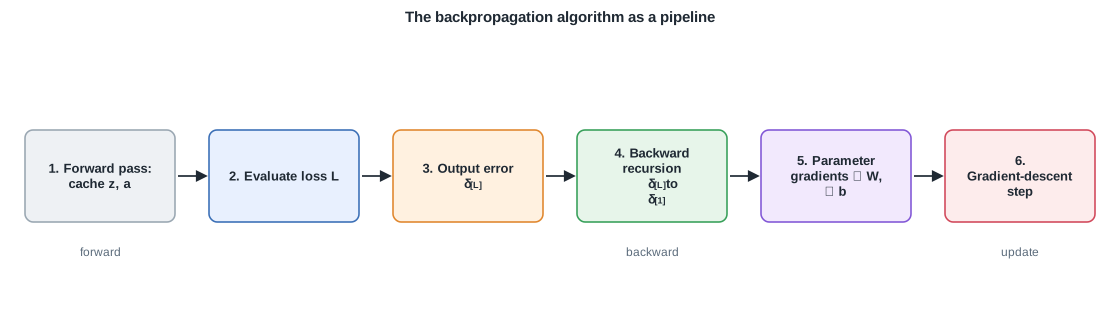
+	Backpropagation runs one forward pass to fill a cache, one backward pass to propagate $\delta$, and then a parameter update.
+
+	1. **Forward pass.** Set $a^{[0]} = x$. For $l = 1, \dots, L$ compute $z^{[l]}$ and $a^{[l]}$, caching each. Evaluate the loss $L$ at $\hat{y} = a^{[L]}$.
+	2. **Output error.** Compute $\delta^{[L]}$ from Section 5.3.
+	3. **Backward pass.** For $l = L-1, \dots, 1$ apply the recursion of Section 5.4 to get $\delta^{[l]}$.
+	4. **Gradients.** For each layer form $\partial L / \partial W^{[l]}$ and $\partial L / \partial b^{[l]}$ from Section 5.5.
+	5. **Update.** Over a batch, average the per-example gradients into the cost gradient $\nabla J$ and take one gradient-descent step (detailed in [Optimization](/en/Deep%20Learning/06%20Optimization)).
+
+	
+
+	*The backpropagation algorithm as a pipeline from a cached forward pass to the parameter update.*
+
+	*Remark:* backpropagation gives the gradient, not the step. It answers which direction lowers the cost, and by how much per unit of each parameter. Turning that gradient into an actual weight change is the job of the optimizer.
+
+	In short, backpropagation is an ordered, single-pass application of the chain rule that reuses cached forward quantities to compute every gradient at the price of roughly one extra forward pass. *With the gradient in hand, the next lesson studies how to use it well: learning rates, momentum, and the adaptive methods that make deep networks trainable.*
+
+	---
+	Next: [Optimization](/en/Deep%20Learning/06%20Optimization) · [Course overview](/en/Deep%20Learning)
/dev/null .. en/Deep Learning/05 Backpropagation/backprop-steps.svg
@@ 0,0 1,1 @@
+	<svg xmlns="http://www.w3.org/2000/svg" viewBox="0 0 1120 320" width="1120" height="320" font-family="Helvetica, Arial, sans-serif"><defs><marker id="arrow" viewBox="0 0 10 10" refX="8.5" refY="5" markerWidth="7" markerHeight="7" orient="auto-start-reverse"><path d="M0 0L10 5L0 10z" fill="#1f2933"/></marker><marker id="arrowmuted" viewBox="0 0 10 10" refX="8.5" refY="5" markerWidth="7" markerHeight="7" orient="auto-start-reverse"><path d="M0 0L10 5L0 10z" fill="#5b6b7b"/></marker></defs><rect width="1120" height="320" fill="#ffffff"/><text x="560.0" y="22.0" font-family="Helvetica, Arial, sans-serif" font-size="15" font-weight="600" fill="#1f2933" text-anchor="middle">The backpropagation algorithm as a pipeline</text><rect x="25.0" y="130.0" width="150.0" height="92.0" rx="8" fill="#eef1f4" stroke="#9aa7b2" stroke-width="1.6"/><text x="100.0" y="172.8" font-family="Helvetica, Arial, sans-serif" font-size="13" font-weight="600" fill="#1f2933" text-anchor="middle">1. Forward pass:</text><text x="100.0" y="188.1" font-family="Helvetica, Arial, sans-serif" font-size="13" font-weight="600" fill="#1f2933" text-anchor="middle">cache z, a</text><rect x="209.0" y="130.0" width="150.0" height="92.0" rx="8" fill="#e8f0fe" stroke="#3b6fb6" stroke-width="1.6"/><text x="284.0" y="180.4" font-family="Helvetica, Arial, sans-serif" font-size="13" font-weight="600" fill="#1f2933" text-anchor="middle">2. Evaluate loss L</text><rect x="393.0" y="130.0" width="150.0" height="92.0" rx="8" fill="#fff1e0" stroke="#e0872e" stroke-width="1.6"/><text x="468.0" y="172.8" font-family="Helvetica, Arial, sans-serif" font-size="13" font-weight="600" fill="#1f2933" text-anchor="middle">3. Output error</text><text x="468.0" y="188.1" font-family="Helvetica, Arial, sans-serif" font-size="13" font-weight="600" fill="#1f2933" text-anchor="middle">δ<tspan baseline-shift="super" font-size="9px">[L]</tspan></text><rect x="577.0" y="130.0" width="150.0" height="92.0" rx="8" fill="#e7f5ea" stroke="#38a05a" stroke-width="1.6"/><text x="652.0" y="157.4" font-family="Helvetica, Arial, sans-serif" font-size="13" font-weight="600" fill="#1f2933" text-anchor="middle">4. Backward</text><text x="652.0" y="172.8" font-family="Helvetica, Arial, sans-serif" font-size="13" font-weight="600" fill="#1f2933" text-anchor="middle">recursion</text><text x="652.0" y="188.1" font-family="Helvetica, Arial, sans-serif" font-size="13" font-weight="600" fill="#1f2933" text-anchor="middle">δ<tspan baseline-shift="super" font-size="9px">[L]</tspan> to</text><text x="652.0" y="203.4" font-family="Helvetica, Arial, sans-serif" font-size="13" font-weight="600" fill="#1f2933" text-anchor="middle">δ<tspan baseline-shift="super" font-size="9px">[1]</tspan></text><rect x="761.0" y="130.0" width="150.0" height="92.0" rx="8" fill="#f2e9fd" stroke="#8257d6" stroke-width="1.6"/><text x="836.0" y="165.1" font-family="Helvetica, Arial, sans-serif" font-size="13" font-weight="600" fill="#1f2933" text-anchor="middle">5. Parameter</text><text x="836.0" y="180.4" font-family="Helvetica, Arial, sans-serif" font-size="13" font-weight="600" fill="#1f2933" text-anchor="middle">gradients ∇ W,</text><text x="836.0" y="195.8" font-family="Helvetica, Arial, sans-serif" font-size="13" font-weight="600" fill="#1f2933" text-anchor="middle">∇ b</text><rect x="945.0" y="130.0" width="150.0" height="92.0" rx="8" fill="#fdecec" stroke="#d1495b" stroke-width="1.6"/><text x="1020.0" y="165.1" font-family="Helvetica, Arial, sans-serif" font-size="13" font-weight="600" fill="#1f2933" text-anchor="middle">6.</text><text x="1020.0" y="180.4" font-family="Helvetica, Arial, sans-serif" font-size="13" font-weight="600" fill="#1f2933" text-anchor="middle">Gradient-descent</text><text x="1020.0" y="195.8" font-family="Helvetica, Arial, sans-serif" font-size="13" font-weight="600" fill="#1f2933" text-anchor="middle">step</text><line x1="178.0" y1="176.0" x2="206.0" y2="176.0" stroke="#1f2933" stroke-width="1.7" marker-end="url(#arrow)"/><line x1="362.0" y1="176.0" x2="390.0" y2="176.0" stroke="#1f2933" stroke-width="1.7" marker-end="url(#arrow)"/><line x1="546.0" y1="176.0" x2="574.0" y2="176.0" stroke="#1f2933" stroke-width="1.7" marker-end="url(#arrow)"/><line x1="730.0" y1="176.0" x2="758.0" y2="176.0" stroke="#1f2933" stroke-width="1.7" marker-end="url(#arrow)"/><line x1="914.0" y1="176.0" x2="942.0" y2="176.0" stroke="#1f2933" stroke-width="1.7" marker-end="url(#arrow)"/><text x="100.0" y="256.0" font-family="Helvetica, Arial, sans-serif" font-size="12" fill="#5b6b7b" text-anchor="middle">forward</text><text x="652.0" y="256.0" font-family="Helvetica, Arial, sans-serif" font-size="12" fill="#5b6b7b" text-anchor="middle">backward</text><text x="1020.0" y="256.0" font-family="Helvetica, Arial, sans-serif" font-size="12" fill="#5b6b7b" text-anchor="middle">update</text></svg>
\	No newline at end of file
/dev/null .. en/Deep Learning/05 Backpropagation/computational-graph.svg
@@ 0,0 1,1 @@
+	<svg xmlns="http://www.w3.org/2000/svg" viewBox="0 0 1080 380" width="1080" height="380" font-family="Helvetica, Arial, sans-serif"><defs><marker id="arrow" viewBox="0 0 10 10" refX="8.5" refY="5" markerWidth="7" markerHeight="7" orient="auto-start-reverse"><path d="M0 0L10 5L0 10z" fill="#1f2933"/></marker><marker id="arrowmuted" viewBox="0 0 10 10" refX="8.5" refY="5" markerWidth="7" markerHeight="7" orient="auto-start-reverse"><path d="M0 0L10 5L0 10z" fill="#5b6b7b"/></marker></defs><rect width="1080" height="380" fill="#ffffff"/><text x="540.0" y="22.0" font-family="Helvetica, Arial, sans-serif" font-size="15" font-weight="600" fill="#1f2933" text-anchor="middle">Forward and backward passes over the computational graph</text><rect x="40.0" y="150.0" width="118.0" height="54.0" rx="8" fill="#eef1f4" stroke="#9aa7b2" stroke-width="1.6"/><text x="99.0" y="182.1" font-family="Helvetica, Arial, sans-serif" font-size="15" font-weight="600" fill="#1f2933" text-anchor="middle">x = a<tspan baseline-shift="super" font-size="11px">[0]</tspan></text><rect x="212.0" y="150.0" width="118.0" height="54.0" rx="8" fill="#e8f0fe" stroke="#3b6fb6" stroke-width="1.6"/><text x="271.0" y="182.1" font-family="Helvetica, Arial, sans-serif" font-size="15" font-weight="600" fill="#1f2933" text-anchor="middle">z<tspan baseline-shift="super" font-size="11px">[1]</tspan></text><rect x="384.0" y="150.0" width="118.0" height="54.0" rx="8" fill="#e7f5ea" stroke="#38a05a" stroke-width="1.6"/><text x="443.0" y="182.1" font-family="Helvetica, Arial, sans-serif" font-size="15" font-weight="600" fill="#1f2933" text-anchor="middle">a<tspan baseline-shift="super" font-size="11px">[1]</tspan></text><rect x="556.0" y="150.0" width="118.0" height="54.0" rx="8" fill="#e8f0fe" stroke="#3b6fb6" stroke-width="1.6"/><text x="615.0" y="182.1" font-family="Helvetica, Arial, sans-serif" font-size="15" font-weight="600" fill="#1f2933" text-anchor="middle">z<tspan baseline-shift="super" font-size="11px">[2]</tspan></text><rect x="728.0" y="150.0" width="118.0" height="54.0" rx="8" fill="#fff1e0" stroke="#e0872e" stroke-width="1.6"/><text x="787.0" y="182.1" font-family="Helvetica, Arial, sans-serif" font-size="15" font-weight="600" fill="#1f2933" text-anchor="middle">ŷ</text><rect x="900.0" y="150.0" width="118.0" height="54.0" rx="8" fill="#fdecec" stroke="#d1495b" stroke-width="1.6"/><text x="959.0" y="182.1" font-family="Helvetica, Arial, sans-serif" font-size="15" font-weight="600" fill="#1f2933" text-anchor="middle">loss L</text><text x="99.0" y="124.0" font-family="Helvetica, Arial, sans-serif" font-size="13" fill="#5b6b7b" text-anchor="start">forward pass (solid): cache z and a</text><line x1="162.0" y1="171.0" x2="208.0" y2="171.0" stroke="#1f2933" stroke-width="1.7" marker-end="url(#arrow)"/><line x1="334.0" y1="171.0" x2="380.0" y2="171.0" stroke="#1f2933" stroke-width="1.7" marker-end="url(#arrow)"/><line x1="506.0" y1="171.0" x2="552.0" y2="171.0" stroke="#1f2933" stroke-width="1.7" marker-end="url(#arrow)"/><line x1="678.0" y1="171.0" x2="724.0" y2="171.0" stroke="#1f2933" stroke-width="1.7" marker-end="url(#arrow)"/><line x1="850.0" y1="171.0" x2="896.0" y2="171.0" stroke="#1f2933" stroke-width="1.7" marker-end="url(#arrow)"/><line x1="959.0" y1="250.0" x2="787.0" y2="250.0" stroke="#5b6b7b" stroke-width="1.7" marker-end="url(#arrowmuted)" stroke-dasharray="5 4"/><text x="873.0" y="242.0" font-family="Helvetica, Arial, sans-serif" font-size="12" fill="#5b6b7b" text-anchor="middle">δ<tspan baseline-shift="super" font-size="9px">[L]</tspan></text><line x1="787.0" y1="250.0" x2="615.0" y2="250.0" stroke="#5b6b7b" stroke-width="1.7" marker-end="url(#arrowmuted)" stroke-dasharray="5 4"/><text x="701.0" y="242.0" font-family="Helvetica, Arial, sans-serif" font-size="12" fill="#5b6b7b" text-anchor="middle">δ<tspan baseline-shift="super" font-size="9px">[2]</tspan></text><line x1="615.0" y1="250.0" x2="443.0" y2="250.0" stroke="#5b6b7b" stroke-width="1.7" marker-end="url(#arrowmuted)" stroke-dasharray="5 4"/><text x="529.0" y="242.0" font-family="Helvetica, Arial, sans-serif" font-size="12" fill="#5b6b7b" text-anchor="middle">∇ W<tspan baseline-shift="super" font-size="9px">[2]</tspan>, ∇ b<tspan baseline-shift="super" font-size="9px">[2]</tspan></text><line x1="443.0" y1="250.0" x2="271.0" y2="250.0" stroke="#5b6b7b" stroke-width="1.7" marker-end="url(#arrowmuted)" stroke-dasharray="5 4"/><text x="357.0" y="242.0" font-family="Helvetica, Arial, sans-serif" font-size="12" fill="#5b6b7b" text-anchor="middle">δ<tspan baseline-shift="super" font-size="9px">[1]</tspan></text><line x1="271.0" y1="250.0" x2="99.0" y2="250.0" stroke="#5b6b7b" stroke-width="1.7" marker-end="url(#arrowmuted)" stroke-dasharray="5 4"/><text x="185.0" y="242.0" font-family="Helvetica, Arial, sans-serif" font-size="12" fill="#5b6b7b" text-anchor="middle">∇ W<tspan baseline-shift="super" font-size="9px">[1]</tspan>, ∇ b<tspan baseline-shift="super" font-size="9px">[1]</tspan></text><text x="99.0" y="280.0" font-family="Helvetica, Arial, sans-serif" font-size="13" fill="#5b6b7b" text-anchor="start">backward pass (dashed): propagate the error δ</text></svg>
\	No newline at end of file
/dev/null .. en/Deep Learning/06 Optimization.md
@@ 0,0 1,133 @@
+	# 6. Optimization
+
+	Backpropagation returns the gradient of the cost with respect to every parameter. An optimizer is the rule that turns those gradients into updates. This module covers the gradient-descent variants and the adaptive optimizers (momentum, RMSProp, Adam) that make deep networks trainable, plus the learning-rate schedules that shape the run.
+
+	**Objectives**
+	- Reuse the gradient-descent update from the Machine Learning course and name its batch, mini-batch, and stochastic variants.
+	- Add momentum to damp oscillations and accelerate along consistent directions.
+	- Rescale each coordinate by its recent gradient magnitude with RMSProp.
+	- Combine both ideas into Adam and understand its bias correction.
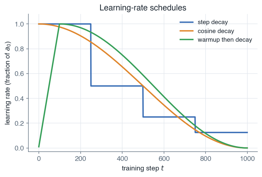
+	- Pick a learning-rate schedule: step decay, cosine, or warmup.
+	- Compare the optimizers and know when to reach for each.
+
+	## 6.1 Gradient descent
+
+	Let $\theta$ collect all parameters (every $W^{[l]}$ and $b^{[l]}$) and let $J(\theta)$ be the cost, the average of the per-example loss $L$. Write $g = \nabla_\theta J(\theta)$ for the gradient of the cost with respect to the parameters, as returned by backpropagation. The base update moves $\theta$ downhill:
+
+	$$\boxed{ \theta \leftarrow \theta - \alpha\, g }$$
+
+	with learning rate $\alpha > 0$. This is the LMS update from the Machine Learning course, written for the full parameter vector instead of one coordinate.
+
+	*Remark:* bias is explicit here. The gradient $g$ has one block per $W^{[l]}$ and one per $b^{[l]}$, and the update applies to each block with the same $\alpha$.
+
+	### 6.1.1 Batch, mini-batch, stochastic
+
+	The variants differ only in how many examples enter the gradient $g$ at each step.
+
+	| variant | examples per step | update noise | per step | use when |
+	| --- | --- | --- | --- | --- |
+	| Batch GD | all $m$ | none | $O(m)$ passes | $m$ small, exact gradient wanted |
+	| Mini-batch GD | a batch of $B$ | moderate | $O(B)$ | the default for deep nets |
+	| Stochastic GD (SGD) | one example | high | $O(1)$ | streaming, very large $m$ |
+
+	*Remark:* one pass over the whole dataset is an epoch. Mini-batch is the standard choice: batches of $32$ to $512$ fit the accelerator, exploit vectorized matrix products, and the residual noise in $g$ helps escape shallow local minima. In deep learning "SGD" is used loosely to mean mini-batch gradient descent.
+
+	## 6.2 Momentum
+
+	Plain SGD zig-zags across narrow valleys because the gradient points across the valley more than along it. Momentum accumulates an exponentially weighted average of past gradients in a velocity vector $v$, then steps in that averaged direction:
+
+	$$\boxed{ v \leftarrow \beta\, v + g, \qquad \theta \leftarrow \theta - \alpha\, v }$$
+
+	with momentum coefficient $\beta \in [0, 1)$, typically $\beta = 0.9$. Components of $g$ that keep the same sign reinforce each other, so $v$ grows and the step accelerates along consistent directions. Components that flip sign cancel in the average, so oscillations across the valley are damped.
+
+	### 6.2.1 Nesterov momentum
+
+	Nesterov accelerated gradient evaluates the gradient at a look-ahead point, after the momentum step has been provisionally applied, rather than at the current $\theta$. This anticipatory correction reacts sooner when the slope changes:
+
+	$$\boxed{ v \leftarrow \beta\, v + \nabla_\theta J(\theta - \alpha \beta\, v), \qquad \theta \leftarrow \theta - \alpha\, v }$$
+
+	*Remark:* think of $\beta \approx 0.9$ as averaging over roughly the last $\tfrac{1}{1 - \beta} = 10$ gradients. Nesterov usually converges slightly faster than plain momentum for the same $\alpha$ and $\beta$.
+
+	## 6.3 RMSProp
+
+	Different parameters can need very different step sizes, and one global $\alpha$ cannot serve them all. RMSProp keeps a per-coordinate running average $s$ of squared gradients, then divides the step by $\sqrt{s}$, so coordinates with large recent gradients take smaller steps and quiet coordinates take larger ones:
+
+	$$\boxed{ s \leftarrow \rho\, s + (1 - \rho)\, g^2, \qquad \theta \leftarrow \theta - \alpha\, \frac{g}{\sqrt{s} + \epsilon} }$$
+
+	with decay $\rho \approx 0.9$ and a small $\epsilon \approx 10^{-8}$ for numerical safety. Here $g^2 = g \odot g$ is the Hadamard (elementwise) square and the division is elementwise, so each coordinate is normalized by its own recent gradient scale.
+
+	*Remark:* $s$ estimates the uncentered second moment of each coordinate of $g$, so $\sqrt{s}$ is roughly its recent root-mean-square magnitude. RMSProp suits non-stationary objectives, which is exactly what a moving mini-batch gradient is.
+
+	## 6.4 Adam
+
+	Adam (adaptive moment estimation) combines momentum and RMSProp: it keeps a first-moment estimate $m$ (the mean of the gradient) and a second-moment estimate $v$ (the mean of the squared gradient).
+
+	$$\boxed{ m \leftarrow \beta_1\, m + (1 - \beta_1)\, g, \qquad v \leftarrow \beta_2\, v + (1 - \beta_2)\, g^2 }$$
+
+	Both $m$ and $v$ start at zero, so early in training they are biased toward zero. Dividing by $1 - \beta_1^t$ and $1 - \beta_2^t$ at step $t$ removes that bias:
+
+	$$\boxed{ \hat m = \frac{m}{1 - \beta_1^{\,t}}, \qquad \hat v = \frac{v}{1 - \beta_2^{\,t}} }$$
+
+	The update then steps in the momentum direction, rescaled per coordinate by the second moment:
+
+	$$\boxed{ \theta \leftarrow \theta - \alpha\, \frac{\hat m}{\sqrt{\hat v} + \epsilon} }$$
+
+	Common defaults are $\beta_1 = 0.9$, $\beta_2 = 0.999$, and $\epsilon = 10^{-8}$. As before the square, square root, and division are elementwise.
+
+	*Remark:* the bias correction matters most in the first few dozen steps, when $t$ is small and $\beta_2^t$ is still close to $1$. Without it, $\hat v$ would be far too small and the early steps far too large. AdamW, a common variant, decouples weight decay from this update.
+
+	
+
+	*Adam combines the momentum of averaged gradients with the per-parameter scaling of RMSProp.*
+
+	## 6.5 Learning-rate schedules
+
+	The learning rate $\alpha$ is the single most important hyperparameter, and holding it fixed is rarely optimal. A large $\alpha$ speeds early progress but prevents settling into a minimum, so schedules typically decrease $\alpha$ over training. Here $\alpha_0$ is the initial rate and $t$ indexes the step or epoch.
+
+	### 6.5.1 Step decay
+
+	Multiply $\alpha$ by a factor $\gamma \in (0, 1)$ every $s$ epochs, so it drops in discrete stages:
+
+	$$\boxed{ \alpha_t = \alpha_0\, \gamma^{\lfloor t / s \rfloor} }$$
+
+	### 6.5.2 Cosine decay
+
+	Anneal $\alpha$ smoothly from $\alpha_0$ toward a floor of zero along a half cosine over $T$ total steps:
+
+	$$\boxed{ \alpha_t = \tfrac{1}{2}\,\alpha_0\left(1 + \cos\frac{\pi t}{T}\right) }$$
+
+	### 6.5.3 Warmup
+
+	Warmup ramps $\alpha$ up linearly from a small value over the first few hundred to few thousand steps, then hands off to a decay schedule. It prevents the large, poorly conditioned updates a cold start with a big $\alpha$ would produce, and it is standard for deep networks such as transformers.
+
+	| schedule | shape | main use |
+	| --- | --- | --- |
+	| Step decay | staircase drops | classic vision training |
+	| Cosine | smooth anneal to zero | modern default, often with warmup |
+	| Warmup | linear ramp up, then decay | stabilize early steps, large models |
+
+	
+
+	*Common learning-rate schedules: step decay, cosine decay, and a warmup followed by decay.*
+
+	*Remark:* warmup and a decay are usually composed, warmup for the first phase and cosine or step decay afterward.
+
+	## 6.6 Choosing an optimizer
+
+	| optimizer | what it adds | tracks | typical use |
+	| --- | --- | --- | --- |
+	| SGD | nothing, base rule | none | strong baseline, best final accuracy with tuning |
+	| Momentum | velocity, damps oscillation | first moment $v$ | vision models, with a schedule |
+	| RMSProp | per-coordinate scaling | second moment $s$ | RNNs, non-stationary objectives |
+	| Adam | momentum plus scaling, bias-corrected | first and second moments | the default first choice for most nets |
+
+	*Remark:* Adam is the safe default and converges fast with little tuning. Well-tuned SGD with momentum and a schedule often reaches slightly better final test accuracy on large vision models, which is why both remain in wide use.
+
+	
+
+	*On an elongated loss surface, momentum and Adam reach the minimum far faster than plain gradient descent.*
+
+	*Every optimizer here scales the raw gradient, so its behaviour depends on how large those gradients are to begin with. The next part studies how the initial weights and the network depth set that scale, and how poor choices make gradients vanish or explode.*
+
+	---
+	Next: [Initialization and vanishing gradients](/en/Deep%20Learning/07%20Initialization%20and%20vanishing%20gradients) · [Course overview](/en/Deep%20Learning)
/dev/null .. en/Deep Learning/06 Optimization/lr-schedules.png
/dev/null .. en/Deep Learning/06 Optimization/optimizer-family.svg
@@ 0,0 1,1 @@
+	<svg xmlns="http://www.w3.org/2000/svg" viewBox="0 0 900 300" width="900" height="300" font-family="Helvetica, Arial, sans-serif"><defs><marker id="arrow" viewBox="0 0 10 10" refX="8.5" refY="5" markerWidth="7" markerHeight="7" orient="auto-start-reverse"><path d="M0 0L10 5L0 10z" fill="#1f2933"/></marker><marker id="arrowmuted" viewBox="0 0 10 10" refX="8.5" refY="5" markerWidth="7" markerHeight="7" orient="auto-start-reverse"><path d="M0 0L10 5L0 10z" fill="#5b6b7b"/></marker></defs><rect width="900" height="300" fill="#ffffff"/><text x="450.0" y="22.0" font-family="Helvetica, Arial, sans-serif" font-size="15" font-weight="600" fill="#1f2933" text-anchor="middle">Adam combines momentum with per-parameter scaling</text><rect x="30.0" y="134.0" width="150.0" height="62.0" rx="8" fill="#eef1f4" stroke="#9aa7b2" stroke-width="1.6"/><text x="105.0" y="162.0" font-family="Helvetica, Arial, sans-serif" font-size="12" fill="#1f2933" text-anchor="middle">gradient g from</text><text x="105.0" y="176.2" font-family="Helvetica, Arial, sans-serif" font-size="12" fill="#1f2933" text-anchor="middle">backprop</text><rect x="270.0" y="60.0" width="190.0" height="62.0" rx="8" fill="#e8f0fe" stroke="#3b6fb6" stroke-width="1.6"/><text x="365.0" y="95.1" font-family="Helvetica, Arial, sans-serif" font-size="12" fill="#1f2933" text-anchor="middle">momentum: average g</text><rect x="270.0" y="200.0" width="190.0" height="62.0" rx="8" fill="#fff1e0" stroke="#e0872e" stroke-width="1.6"/><text x="365.0" y="235.1" font-family="Helvetica, Arial, sans-serif" font-size="12" fill="#1f2933" text-anchor="middle">RMSProp: scale by g<tspan baseline-shift="super" font-size="9px">2</tspan></text><rect x="510.0" y="134.0" width="170.0" height="62.0" rx="8" fill="#e7f5ea" stroke="#38a05a" stroke-width="1.6"/><text x="595.0" y="169.4" font-family="Helvetica, Arial, sans-serif" font-size="13" font-weight="600" fill="#1f2933" text-anchor="middle">Adam combines both</text><rect x="730.0" y="134.0" width="150.0" height="62.0" rx="8" fill="#f2e9fd" stroke="#8257d6" stroke-width="1.6"/><text x="805.0" y="169.1" font-family="Helvetica, Arial, sans-serif" font-size="12" fill="#1f2933" text-anchor="middle">parameter update</text><path d="M180.0 157.0 Q225.0 91.0 270.0 91.0" fill="none" stroke="#1f2933" stroke-width="1.7" marker-end="url(#arrow)"/><path d="M180.0 173.0 Q225.0 231.0 270.0 231.0" fill="none" stroke="#1f2933" stroke-width="1.7" marker-end="url(#arrow)"/><path d="M460.0 91.0 Q485.0 157.0 510.0 157.0" fill="none" stroke="#1f2933" stroke-width="1.7" marker-end="url(#arrow)"/><path d="M460.0 231.0 Q485.0 173.0 510.0 173.0" fill="none" stroke="#1f2933" stroke-width="1.7" marker-end="url(#arrow)"/><line x1="680.0" y1="165.0" x2="730.0" y2="165.0" stroke="#1f2933" stroke-width="1.7" marker-end="url(#arrow)"/></svg>
\	No newline at end of file
/dev/null .. en/Deep Learning/06 Optimization/optimizer-paths.png
/dev/null .. en/Deep Learning/07 Initialization and vanishing gradients.md
@@ 0,0 1,117 @@
+	# 7. Initialization and vanishing gradients
+
+	Deep networks are hard to train because backpropagation multiplies one Jacobian per layer, so a signal can shrink or blow up geometrically with depth. This module explains where that instability comes from, why naive weight initialization makes it worse, and the two fixes that make deep training routine: variance-preserving initialization (Xavier and He) and gradient clipping.
+
+	**Objectives**
+	- Write backpropagation as a product of per-layer Jacobians and see when it vanishes or explodes.
+	- Connect the effect to activation saturation from lesson 3.
+	- Explain why all-zeros and badly scaled initializations fail.
+	- Derive the variance target that Xavier and He initialization satisfy.
+	- Apply gradient clipping to tame exploding gradients.
+	- Pick an initializer from the activation function.
+
+	## 7.1 Why depth is unstable
+
+	### 7.1.1 The Jacobian product
+
+	Recall the forward pass of lesson 6: layer $l$ computes $z^{[l]} = W^{[l]} a^{[l-1]} + b^{[l]}$ and $a^{[l]} = g^{[l]}(z^{[l]})$, with $a^{[0]} = x$ and $\hat{y} = a^{[L]}$. Backpropagation sends the loss gradient from the output back to layer $l$ by the chain rule. The error signal $\delta^{[l]} = \partial L / \partial z^{[l]}$ obeys the recurrence $\delta^{[l]} = (W^{[l+1]})^T \delta^{[l+1]} \odot g'^{[l]}(z^{[l]})$, so unrolling it from the top layer $L$ down to layer $l$ gives a product:
+
+	$$\boxed{ \frac{\partial L}{\partial z^{[l]}} = \left( \prod_{k=l+1}^{L} \operatorname{diag}\!\left(g'^{[k-1]}(z^{[k-1]})\right) (W^{[k]})^T \right) \frac{\partial L}{\partial z^{[L]}} }$$
+
+	Each factor is a layer Jacobian: a weight matrix $W^{[k]}$ combined with the diagonal matrix $\operatorname{diag}(g'(z))$ of activation slopes. The gradient reaching layer $l$ is this whole product acting on the top-layer error.
+
+	### 7.1.2 Vanishing and exploding
+
+	A product of many factors is governed by their typical magnitude. Write $\rho$ for the typical size (a spectral norm) of one factor $W^{[k]} \odot \operatorname{diag}(g')$. Across $L - l$ layers the signal scales roughly as $\rho^{\,L-l}$:
+
+	$$\boxed{ \left\| \frac{\partial L}{\partial z^{[l]}} \right\| \;\approx\; \rho^{\,L-l} \left\| \frac{\partial L}{\partial z^{[L]}} \right\| }$$
+
+	If $\rho < 1$ consistently the gradient shrinks toward zero as it travels back (the **vanishing gradient**), so early layers barely update and effectively stop learning. If $\rho > 1$ it grows without bound (the **exploding gradient**), so updates overshoot and the loss diverges to `NaN`. Only $\rho \approx 1$ keeps the signal alive across depth.
+
+	
+
+	*Gradient magnitude across depth: poorly scaled weights make it vanish or explode, while variance-preserving initialization keeps it near one.*
+
+	*Remark:* the same product runs forward for the activations themselves. If layer outputs shrink or grow geometrically, the network cannot represent anything useful even before a gradient is computed, so we want both the forward signal and the backward gradient near unit scale.
+
+	### 7.1.3 The saturation connection
+
+	The factor $g'(z)$ links this directly to the saturation seen in lesson 3. The sigmoid and $\tanh$ flatten for large $|z|$, so their derivatives fall to near zero there.
+
+	| Activation | $g'(z)$ | max slope | slope when saturated |
+	| --- | --- | --- | --- |
+	| sigmoid | $g(z)(1-g(z))$ | $0.25$ | $\to 0$ |
+	| $\tanh$ | $1 - \tanh^2(z)$ | $1$ | $\to 0$ |
+	| ReLU | $1$ for $z>0$, else $0$ | $1$ | $0$ on the dead side |
+
+	*Remark:* the sigmoid slope never exceeds $0.25$, so each layer multiplies the backward signal by at most a quarter. Stack ten sigmoid layers and the gradient is scaled by at most $0.25^{10} \approx 10^{-6}$ before any weight is considered. This is why deep stacks of saturating units train poorly, and why ReLU (slope $1$ on the active side) became the default.
+
+	## 7.2 Bad initializations
+
+	### 7.2.1 All zeros
+
+	Setting $W^{[l]} = 0$ (or any value that makes every unit in a layer identical) breaks learning through **symmetry**. If two units in a layer start with the same weights and see the same input, they compute the same activation and receive the same gradient, so they update identically and stay identical forever. The layer then behaves like a single unit no matter how wide it is. Random initialization exists precisely to break this symmetry so units can specialize.
+
+	### 7.2.2 Wrong scale
+
+	Even with random, symmetry-breaking weights the **variance** matters. Consider a linear unit $z = \sum_{j=1}^{n_{\text{in}}} W_j a_j$ with independent zero-mean weights and inputs. Its variance is a sum of $n_{\text{in}}$ independent terms:
+
+	$$\boxed{ \operatorname{Var}(z) = n_{\text{in}} \cdot \operatorname{Var}(W) \cdot \operatorname{Var}(a) }$$
+
+	If $n_{\text{in}} \cdot \operatorname{Var}(W) > 1$ the signal variance grows layer after layer and explodes, and if it is $< 1$ the variance decays and vanishes. To keep $\operatorname{Var}(z) \approx \operatorname{Var}(a)$ from layer to layer we need $n_{\text{in}} \cdot \operatorname{Var}(W) \approx 1$, which fixes the weight variance to roughly $1 / n_{\text{in}}$. That single condition is the seed of both initializers below.
+
+	## 7.3 Variance-preserving initialization
+
+	### 7.3.1 Xavier / Glorot
+
+	Glorot and Bengio balance the forward pass ($\operatorname{Var}(W) = 1/n_{\text{in}}$) against the backward pass ($\operatorname{Var}(W) = 1/n_{\text{out}}$) by averaging the two, giving the Xavier initialization:
+
+	$$\boxed{ \operatorname{Var}(W^{[l]}) = \frac{2}{n_{\text{in}} + n_{\text{out}}} }$$
+
+	Here $n_{\text{in}} = n_{l-1}$ is the fan-in and $n_{\text{out}} = n_l$ is the fan-out of the layer. Xavier is derived assuming the activation is roughly linear near the origin, so it suits **symmetric, unit-slope** activations like $\tanh$ and the sigmoid.
+
+	### 7.3.2 He
+
+	ReLU zeros out half of its inputs on average, so it halves the variance of what passes through. He initialization compensates with a factor of two:
+
+	$$\boxed{ \operatorname{Var}(W^{[l]}) = \frac{2}{n_{\text{in}}} }$$
+
+	This is the right target for **ReLU and its variants** (leaky ReLU, ELU, GELU). In practice you draw weights from a Gaussian with this variance, or from a uniform distribution with the matching range, and set the bias $b^{[l]}$ to zero.
+
+	*Remark:* the bias starts at zero, not the weights. A zero bias does not create symmetry (the weights already differ), and it keeps the initial pre-activation centred so the activation starts in its responsive region rather than saturated.
+
+	### 7.3.3 The mechanism
+
+	
+
+	*Variance-preserving initialization keeps the signal and the gradient near unit scale through depth.*
+
+	Choosing the variance is a one-time fix at the start of training. It positions the network so the Jacobian product of section 7.1 has factors near $1$, but nothing keeps it there as the weights move during training. That is what the next module addresses.
+
+	## 7.4 Exploding gradients and clipping
+
+	Good initialization tames vanishing gradients and greatly reduces explosions, but explosions can still appear during training, especially in recurrent networks where the same weight matrix is reused at every time step. The standard remedy is **gradient clipping**: rescale the whole gradient vector $g$ so its norm never exceeds a threshold $\tau$.
+
+	$$\boxed{ g \leftarrow g \cdot \min\!\left(1, \frac{\tau}{\lVert g \rVert}\right) }$$
+
+	When $\lVert g \rVert \le \tau$ the factor is $1$ and the gradient is untouched. When $\lVert g \rVert > \tau$ the gradient is shrunk back to norm exactly $\tau$ while keeping its direction, so a single huge step cannot blow up the weights.
+
+	*Remark:* clipping by global norm (rescaling the whole vector together) preserves the update direction, whereas clipping each coordinate independently to $[-\tau, \tau]$ can bend the direction. Global-norm clipping is the usual default.
+
+	## 7.5 Choosing an initializer
+
+	Match the initializer to the activation of the layer it feeds.
+
+	| Activation | Recommended initializer | Weight variance |
+	| --- | --- | --- |
+	| ReLU, leaky ReLU, ELU, GELU | He | $2 / n_{\text{in}}$ |
+	| $\tanh$ | Xavier / Glorot | $2 / (n_{\text{in}} + n_{\text{out}})$ |
+	| sigmoid | Xavier / Glorot | $2 / (n_{\text{in}} + n_{\text{out}})$ |
+	| softmax / linear output | Xavier / Glorot | $2 / (n_{\text{in}} + n_{\text{out}})$ |
+
+	*Remark:* initialization and clipping only manage the signal at the endpoints of training and during large steps. Two structural remedies keep it controlled throughout: **normalization** re-centres and rescales activations at every layer, and **residual connections** add a shortcut that lets the gradient skip past the Jacobian product entirely.
+
+	*Good initialization keeps the signal well scaled at step zero, but the statistics drift as training proceeds. The next module keeps them in check at every step with normalization.*
+
+	---
+	Next: [Normalization](/en/Deep%20Learning/08%20Normalization) · [Course overview](/en/Deep%20Learning)
/dev/null .. en/Deep Learning/07 Initialization and vanishing gradients/gradient-flow.png
/dev/null .. en/Deep Learning/07 Initialization and vanishing gradients/init-reasoning.svg
@@ 0,0 1,1 @@
+	<svg xmlns="http://www.w3.org/2000/svg" viewBox="0 0 1080 190" width="1080" height="190" font-family="Helvetica, Arial, sans-serif"><defs><marker id="arrow" viewBox="0 0 10 10" refX="8.5" refY="5" markerWidth="7" markerHeight="7" orient="auto-start-reverse"><path d="M0 0L10 5L0 10z" fill="#1f2933"/></marker><marker id="arrowmuted" viewBox="0 0 10 10" refX="8.5" refY="5" markerWidth="7" markerHeight="7" orient="auto-start-reverse"><path d="M0 0L10 5L0 10z" fill="#5b6b7b"/></marker></defs><rect width="1080" height="190" fill="#ffffff"/><text x="540.0" y="22.0" font-family="Helvetica, Arial, sans-serif" font-size="15" font-weight="600" fill="#1f2933" text-anchor="middle">Why variance-preserving initialization stabilizes depth</text><rect x="24.0" y="78.0" width="176.0" height="66.0" rx="8" fill="#f2e9fd" stroke="#8257d6" stroke-width="1.6"/><text x="112.0" y="107.8" font-family="Helvetica, Arial, sans-serif" font-size="13" fill="#1f2933" text-anchor="middle">random W break</text><text x="112.0" y="123.1" font-family="Helvetica, Arial, sans-serif" font-size="13" fill="#1f2933" text-anchor="middle">symmetry</text><rect x="224.0" y="78.0" width="176.0" height="66.0" rx="8" fill="#e8f0fe" stroke="#3b6fb6" stroke-width="1.6"/><text x="312.0" y="107.8" font-family="Helvetica, Arial, sans-serif" font-size="13" fill="#1f2933" text-anchor="middle">set Var(W) near</text><text x="312.0" y="123.1" font-family="Helvetica, Arial, sans-serif" font-size="13" fill="#1f2933" text-anchor="middle">1/n<tspan baseline-shift="sub" font-size="9px">in</tspan></text><rect x="424.0" y="78.0" width="176.0" height="66.0" rx="8" fill="#e4f5f4" stroke="#2a9d9a" stroke-width="1.6"/><text x="512.0" y="107.8" font-family="Helvetica, Arial, sans-serif" font-size="13" fill="#1f2933" text-anchor="middle">signal Var(z) near</text><text x="512.0" y="123.1" font-family="Helvetica, Arial, sans-serif" font-size="13" fill="#1f2933" text-anchor="middle">Var(a)</text><rect x="624.0" y="78.0" width="176.0" height="66.0" rx="8" fill="#e7f5ea" stroke="#38a05a" stroke-width="1.6"/><text x="712.0" y="107.8" font-family="Helvetica, Arial, sans-serif" font-size="13" fill="#1f2933" text-anchor="middle">gradient factor ρ</text><text x="712.0" y="123.1" font-family="Helvetica, Arial, sans-serif" font-size="13" fill="#1f2933" text-anchor="middle">near 1</text><rect x="824.0" y="78.0" width="176.0" height="66.0" rx="8" fill="#fff1e0" stroke="#e0872e" stroke-width="1.6"/><text x="912.0" y="107.8" font-family="Helvetica, Arial, sans-serif" font-size="13" fill="#1f2933" text-anchor="middle">deep network trains</text><text x="912.0" y="123.1" font-family="Helvetica, Arial, sans-serif" font-size="13" fill="#1f2933" text-anchor="middle">stably</text><line x1="200.0" y1="111.0" x2="224.0" y2="111.0" stroke="#1f2933" stroke-width="1.7" marker-end="url(#arrow)"/><line x1="400.0" y1="111.0" x2="424.0" y2="111.0" stroke="#1f2933" stroke-width="1.7" marker-end="url(#arrow)"/><line x1="600.0" y1="111.0" x2="624.0" y2="111.0" stroke="#1f2933" stroke-width="1.7" marker-end="url(#arrow)"/><line x1="800.0" y1="111.0" x2="824.0" y2="111.0" stroke="#1f2933" stroke-width="1.7" marker-end="url(#arrow)"/></svg>
\	No newline at end of file
/dev/null .. en/Deep Learning/08 Normalization.md
@@ 0,0 1,122 @@
+	# 8. Normalization
+
+	Deep networks train faster and more reliably when the activations flowing between layers stay well-scaled. This lesson introduces normalization layers, which standardize a layer's inputs on the fly, then learn to rescale them. We cover batch normalization and layer normalization, where each computes its statistics, how they behave at inference, and where to place them.
+
+	**Objectives**
+	- Explain why normalizing activations inside the network stabilizes and accelerates training.
+	- Derive the batch normalization transform: normalize, then scale and shift with learned $\gamma, \beta$.
+	- Understand why running (moving-average) statistics replace batch statistics at inference.
+	- Define layer normalization and see why it suits recurrent networks and Transformers.
+	- Decide where to place a normalization layer relative to the activation $g^{[l]}$.
+	- Compare batch and layer normalization along their normalization axis and use cases.
+
+	## 8.1 Why normalize inside the network
+
+	Recall a layer computes $z^{[l]} = W^{[l]} a^{[l-1]} + b^{[l]}$ and $a^{[l]} = g^{[l]}(z^{[l]})$. As training updates every $W^{[l]}$, the distribution of each layer's input $a^{[l-1]}$ keeps shifting. This moving target, sometimes called internal covariate shift, forces later layers to constantly re-adapt and slows the whole network down.
+
+	Normalizing the activations at each layer keeps their mean and variance stable across updates. The immediate benefits:
+
+	- The loss surface becomes smoother, so we can use a higher learning rate without diverging.
+	- Training converges in fewer epochs and is less sensitive to the weight initialization.
+	- The learned scale and shift give the network back the freedom to undo the normalization if that helps.
+
+	*Remark:* normalization is applied to the pre-activation $z^{[l]}$ or the activation $a^{[l]}$, not to the parameters. It is a layer inserted into the forward pass, with its own learnable parameters.
+
+	## 8.2 Batch normalization
+
+	Batch normalization (BatchNorm) standardizes each feature across the examples of a mini-batch, then applies a learned affine transform. It operates per feature, so every feature keeps its own statistics.
+
+	
+
+	*Normalization recenters and rescales a layer input to zero mean and unit variance before the learned scale and shift.*
+
+	### 8.2.1 Batch statistics
+
+	For a feature $x$ over a mini-batch $\mathcal{B} = \{x^{(1)}, \dots, x^{(m)}\}$ of size $m$, compute the batch mean and variance:
+
+	$$\boxed{ \mu_\mathcal{B} = \frac{1}{m}\sum_{i=1}^{m} x^{(i)}, \qquad \sigma_\mathcal{B}^2 = \frac{1}{m}\sum_{i=1}^{m}\left(x^{(i)} - \mu_\mathcal{B}\right)^2 }$$
+
+	### 8.2.2 Normalize, scale, and shift
+
+	Standardize each value to zero mean and unit variance, using a small constant $\epsilon > 0$ for numerical stability:
+
+	$$\boxed{ \hat{x}^{(i)} = \frac{x^{(i)} - \mu_\mathcal{B}}{\sqrt{\sigma_\mathcal{B}^2 + \epsilon}} }$$
+
+	Then rescale with two learned parameters per feature, a scale $\gamma$ and a shift $\beta$:
+
+	$$\boxed{ y^{(i)} = \gamma\, \hat{x}^{(i)} + \beta }$$
+
+	*Remark:* $\gamma$ and $\beta$ are learned by gradient descent like any weight. If the optimal behaviour is the raw input, the network can recover it by learning $\gamma = \sqrt{\sigma_\mathcal{B}^2 + \epsilon}$ and $\beta = \mu_\mathcal{B}$. Normalization never removes capacity, it only reparameterizes it.
+
+	### 8.2.3 Inference with running statistics
+
+	At inference we often score a single example, so a batch mean and variance are undefined or meaningless. Instead BatchNorm uses population estimates accumulated during training as exponential moving averages, with momentum $\alpha \in [0, 1)$:
+
+	$$\boxed{ \mu \leftarrow \alpha\, \mu + (1 - \alpha)\, \mu_\mathcal{B}, \qquad \sigma^2 \leftarrow \alpha\, \sigma^2 + (1 - \alpha)\, \sigma_\mathcal{B}^2 }$$
+
+	At test time the transform is fixed and deterministic, using these running statistics in place of the batch ones:
+
+	$$\boxed{ y = \gamma\, \frac{x - \mu}{\sqrt{\sigma^2 + \epsilon}} + \beta }$$
+
+	*Remark:* this train/inference split is the source of most BatchNorm bugs. Forgetting to switch the layer to evaluation mode leaves it computing batch statistics at test time, which corrupts predictions.
+
+	## 8.3 Layer normalization
+
+	Layer normalization (LayerNorm) keeps the same normalize-scale-shift recipe but changes the axis it averages over. Rather than pooling across the batch, it computes the statistics over the features of a single example. Each example is therefore normalized on its own, independent of the others in the batch.
+
+	### 8.3.1 Per-example statistics
+
+	For one example with feature vector $a \in \mathbb{R}^{H}$ (its $H$ activations in a layer), average over the features:
+
+	$$\boxed{ \mu = \frac{1}{H}\sum_{k=1}^{H} a_k, \qquad \sigma^2 = \frac{1}{H}\sum_{k=1}^{H}\left(a_k - \mu\right)^2 }$$
+
+	The normalization, scale, and shift are identical in form to BatchNorm, applied per example:
+
+	$$\boxed{ \hat{a}_k = \frac{a_k - \mu}{\sqrt{\sigma^2 + \epsilon}}, \qquad y_k = \gamma_k\, \hat{a}_k + \beta_k }$$
+
+	### 8.3.2 Why LayerNorm for sequences
+
+	Because the statistics come from a single example, LayerNorm behaves the same in training and inference, and it does not depend on the batch size. This matters when the batch is tiny or when examples have variable length, as in text. LayerNorm is the normalization of choice for recurrent networks and Transformers, where the sequence length varies and a per-timestep batch mean would be ill-defined.
+
+	*Remark:* LayerNorm needs no running statistics, so there is no train/inference discrepancy to manage. This alone makes it simpler to deploy than BatchNorm.
+
+	## 8.4 Placement and practical effects
+
+	A normalization layer sits between the linear step $W^{[l]} a^{[l-1]} + b^{[l]}$ and the nonlinearity $g^{[l]}$. Two orderings are common.
+
+	
+
+	*Normalization is inserted between the linear map and the activation inside each layer.*
+
+	- **Before activation** (normalize $z^{[l]}$, then apply $g^{[l]}$): the original and most common placement. It keeps the input to the nonlinearity centred, which is where saturation hurts most.
+	- **After activation** (normalize $a^{[l]}$): sometimes used and occasionally better in practice, though it is less standard.
+
+	Two more practical points:
+
+	- **Bias becomes redundant.** The shift $\beta$ replaces the layer bias, since normalization subtracts the mean and would cancel $b^{[l]}$ anyway. Layers followed by normalization are often written without their own bias.
+	- **BatchNorm depends on batch size.** Its statistics are noisier with small batches, which acts as a mild regularizer but degrades badly when the batch is very small. LayerNorm is immune to this, which is another reason sequence models prefer it.
+
+	*Remark:* the batch-dependent noise in BatchNorm can partly substitute for other regularizers, so networks using it sometimes need less dropout.
+
+	## 8.5 BatchNorm versus LayerNorm
+
+	The two layers share the normalize-scale-shift transform and differ only in the axis of the statistics and the consequences that follow.
+
+	| Aspect | Batch normalization | Layer normalization |
+	| --- | --- | --- |
+	| Normalization axis | across the batch, per feature | across the features, per example |
+	| Depends on batch size | yes | no |
+	| Train vs inference | batch statistics vs running statistics | identical in both |
+	| Running statistics needed | yes | no |
+	| Typical use | CNNs and feedforward vision models | RNNs and Transformers |
+
+	
+
+	*Batch normalization computes statistics down a feature column across the batch, layer normalization across the features of a single example.*
+
+	*Remark:* the Transformer block in lesson 16 places a LayerNorm before or after each sublayer, precisely because it removes the batch dependence that would otherwise couple examples of different lengths.
+
+	*With activations kept well-scaled, the network trains stably at higher learning rates. The next lesson turns to controlling overfitting through regularization and dropout.*
+
+	---
+	Next: [Regularization and dropout](/en/Deep%20Learning/09%20Regularization%20and%20dropout) · [Course overview](/en/Deep%20Learning)
/dev/null .. en/Deep Learning/08 Normalization/batchnorm-vs-layernorm.svg
@@ 0,0 1,1 @@
+	<svg xmlns="http://www.w3.org/2000/svg" viewBox="0 0 694 350" width="694" height="350" font-family="Helvetica, Arial, sans-serif"><defs><marker id="arrow" viewBox="0 0 10 10" refX="8.5" refY="5" markerWidth="7" markerHeight="7" orient="auto-start-reverse"><path d="M0 0L10 5L0 10z" fill="#1f2933"/></marker><marker id="arrowmuted" viewBox="0 0 10 10" refX="8.5" refY="5" markerWidth="7" markerHeight="7" orient="auto-start-reverse"><path d="M0 0L10 5L0 10z" fill="#5b6b7b"/></marker></defs><rect width="694" height="350" fill="#ffffff"/><text x="330.0" y="22.0" font-family="Helvetica, Arial, sans-serif" font-size="15" font-weight="600" fill="#1f2933" text-anchor="middle">Where each normalization computes its statistics</text><rect x="90.0" y="90.0" width="40.0" height="40.0" rx="4" fill="#eef1f4" stroke="#9aa7b2" stroke-width="1.4"/><rect x="130.0" y="90.0" width="40.0" height="40.0" rx="4" fill="#eef1f4" stroke="#9aa7b2" stroke-width="1.4"/><rect x="170.0" y="90.0" width="40.0" height="40.0" rx="4" fill="#e4f5f4" stroke="#2a9d9a" stroke-width="1.4"/><rect x="210.0" y="90.0" width="40.0" height="40.0" rx="4" fill="#eef1f4" stroke="#9aa7b2" stroke-width="1.4"/><rect x="250.0" y="90.0" width="40.0" height="40.0" rx="4" fill="#eef1f4" stroke="#9aa7b2" stroke-width="1.4"/><rect x="90.0" y="130.0" width="40.0" height="40.0" rx="4" fill="#eef1f4" stroke="#9aa7b2" stroke-width="1.4"/><rect x="130.0" y="130.0" width="40.0" height="40.0" rx="4" fill="#eef1f4" stroke="#9aa7b2" stroke-width="1.4"/><rect x="170.0" y="130.0" width="40.0" height="40.0" rx="4" fill="#e4f5f4" stroke="#2a9d9a" stroke-width="1.4"/><rect x="210.0" y="130.0" width="40.0" height="40.0" rx="4" fill="#eef1f4" stroke="#9aa7b2" stroke-width="1.4"/><rect x="250.0" y="130.0" width="40.0" height="40.0" rx="4" fill="#eef1f4" stroke="#9aa7b2" stroke-width="1.4"/><rect x="90.0" y="170.0" width="40.0" height="40.0" rx="4" fill="#eef1f4" stroke="#9aa7b2" stroke-width="1.4"/><rect x="130.0" y="170.0" width="40.0" height="40.0" rx="4" fill="#eef1f4" stroke="#9aa7b2" stroke-width="1.4"/><rect x="170.0" y="170.0" width="40.0" height="40.0" rx="4" fill="#e4f5f4" stroke="#2a9d9a" stroke-width="1.4"/><rect x="210.0" y="170.0" width="40.0" height="40.0" rx="4" fill="#eef1f4" stroke="#9aa7b2" stroke-width="1.4"/><rect x="250.0" y="170.0" width="40.0" height="40.0" rx="4" fill="#eef1f4" stroke="#9aa7b2" stroke-width="1.4"/><rect x="90.0" y="210.0" width="40.0" height="40.0" rx="4" fill="#eef1f4" stroke="#9aa7b2" stroke-width="1.4"/><rect x="130.0" y="210.0" width="40.0" height="40.0" rx="4" fill="#eef1f4" stroke="#9aa7b2" stroke-width="1.4"/><rect x="170.0" y="210.0" width="40.0" height="40.0" rx="4" fill="#e4f5f4" stroke="#2a9d9a" stroke-width="1.4"/><rect x="210.0" y="210.0" width="40.0" height="40.0" rx="4" fill="#eef1f4" stroke="#9aa7b2" stroke-width="1.4"/><rect x="250.0" y="210.0" width="40.0" height="40.0" rx="4" fill="#eef1f4" stroke="#9aa7b2" stroke-width="1.4"/><text x="190.0" y="60.0" font-family="Helvetica, Arial, sans-serif" font-size="14" font-weight="600" fill="#1f2933" text-anchor="middle">Batch normalization</text><text x="190.0" y="78.0" font-family="Helvetica, Arial, sans-serif" font-size="12" fill="#5b6b7b" text-anchor="middle">stats over the batch, per feature</text><text x="68.0" y="170.0" font-family="Helvetica, Arial, sans-serif" font-size="12" fill="#5b6b7b" text-anchor="middle">examples</text><text x="190.0" y="276.0" font-family="Helvetica, Arial, sans-serif" font-size="12" fill="#5b6b7b" text-anchor="middle">features</text><line x1="190.0" y1="294.0" x2="190.0" y2="310.0" stroke="#5b6b7b" stroke-width="1.7" marker-end="url(#arrowmuted)"/><text x="190.0" y="297.0" font-family="Helvetica, Arial, sans-serif" font-size="11" fill="#5b6b7b" text-anchor="middle">down a column</text><rect x="420.0" y="90.0" width="40.0" height="40.0" rx="4" fill="#eef1f4" stroke="#9aa7b2" stroke-width="1.4"/><rect x="460.0" y="90.0" width="40.0" height="40.0" rx="4" fill="#eef1f4" stroke="#9aa7b2" stroke-width="1.4"/><rect x="500.0" y="90.0" width="40.0" height="40.0" rx="4" fill="#eef1f4" stroke="#9aa7b2" stroke-width="1.4"/><rect x="540.0" y="90.0" width="40.0" height="40.0" rx="4" fill="#eef1f4" stroke="#9aa7b2" stroke-width="1.4"/><rect x="580.0" y="90.0" width="40.0" height="40.0" rx="4" fill="#eef1f4" stroke="#9aa7b2" stroke-width="1.4"/><rect x="420.0" y="130.0" width="40.0" height="40.0" rx="4" fill="#e4f5f4" stroke="#2a9d9a" stroke-width="1.4"/><rect x="460.0" y="130.0" width="40.0" height="40.0" rx="4" fill="#e4f5f4" stroke="#2a9d9a" stroke-width="1.4"/><rect x="500.0" y="130.0" width="40.0" height="40.0" rx="4" fill="#e4f5f4" stroke="#2a9d9a" stroke-width="1.4"/><rect x="540.0" y="130.0" width="40.0" height="40.0" rx="4" fill="#e4f5f4" stroke="#2a9d9a" stroke-width="1.4"/><rect x="580.0" y="130.0" width="40.0" height="40.0" rx="4" fill="#e4f5f4" stroke="#2a9d9a" stroke-width="1.4"/><rect x="420.0" y="170.0" width="40.0" height="40.0" rx="4" fill="#eef1f4" stroke="#9aa7b2" stroke-width="1.4"/><rect x="460.0" y="170.0" width="40.0" height="40.0" rx="4" fill="#eef1f4" stroke="#9aa7b2" stroke-width="1.4"/><rect x="500.0" y="170.0" width="40.0" height="40.0" rx="4" fill="#eef1f4" stroke="#9aa7b2" stroke-width="1.4"/><rect x="540.0" y="170.0" width="40.0" height="40.0" rx="4" fill="#eef1f4" stroke="#9aa7b2" stroke-width="1.4"/><rect x="580.0" y="170.0" width="40.0" height="40.0" rx="4" fill="#eef1f4" stroke="#9aa7b2" stroke-width="1.4"/><rect x="420.0" y="210.0" width="40.0" height="40.0" rx="4" fill="#eef1f4" stroke="#9aa7b2" stroke-width="1.4"/><rect x="460.0" y="210.0" width="40.0" height="40.0" rx="4" fill="#eef1f4" stroke="#9aa7b2" stroke-width="1.4"/><rect x="500.0" y="210.0" width="40.0" height="40.0" rx="4" fill="#eef1f4" stroke="#9aa7b2" stroke-width="1.4"/><rect x="540.0" y="210.0" width="40.0" height="40.0" rx="4" fill="#eef1f4" stroke="#9aa7b2" stroke-width="1.4"/><rect x="580.0" y="210.0" width="40.0" height="40.0" rx="4" fill="#eef1f4" stroke="#9aa7b2" stroke-width="1.4"/><text x="520.0" y="60.0" font-family="Helvetica, Arial, sans-serif" font-size="14" font-weight="600" fill="#1f2933" text-anchor="middle">Layer normalization</text><text x="520.0" y="78.0" font-family="Helvetica, Arial, sans-serif" font-size="12" fill="#5b6b7b" text-anchor="middle">stats over the features, per example</text><text x="398.0" y="170.0" font-family="Helvetica, Arial, sans-serif" font-size="12" fill="#5b6b7b" text-anchor="middle">examples</text><text x="520.0" y="276.0" font-family="Helvetica, Arial, sans-serif" font-size="12" fill="#5b6b7b" text-anchor="middle">features</text><line x1="628.0" y1="150.0" x2="648.0" y2="150.0" stroke="#5b6b7b" stroke-width="1.7" marker-end="url(#arrowmuted)"/><text x="638.0" y="145.0" font-family="Helvetica, Arial, sans-serif" font-size="11" fill="#5b6b7b" text-anchor="middle">across a row</text></svg>
\	No newline at end of file
/dev/null .. en/Deep Learning/08 Normalization/norm-placement.svg
@@ 0,0 1,1 @@
+	<svg xmlns="http://www.w3.org/2000/svg" viewBox="0 0 760 200" width="760" height="200" font-family="Helvetica, Arial, sans-serif"><defs><marker id="arrow" viewBox="0 0 10 10" refX="8.5" refY="5" markerWidth="7" markerHeight="7" orient="auto-start-reverse"><path d="M0 0L10 5L0 10z" fill="#1f2933"/></marker><marker id="arrowmuted" viewBox="0 0 10 10" refX="8.5" refY="5" markerWidth="7" markerHeight="7" orient="auto-start-reverse"><path d="M0 0L10 5L0 10z" fill="#5b6b7b"/></marker></defs><rect width="760" height="200" fill="#ffffff"/><text x="380.0" y="22.0" font-family="Helvetica, Arial, sans-serif" font-size="15" font-weight="600" fill="#1f2933" text-anchor="middle">Normalization inside a layer</text><rect x="40.0" y="90.0" width="150.0" height="60.0" rx="8" fill="#e8f0fe" stroke="#3b6fb6" stroke-width="1.6"/><text x="115.0" y="124.4" font-family="Helvetica, Arial, sans-serif" font-size="13" fill="#1f2933" text-anchor="middle">linear W a + b</text><rect x="210.0" y="90.0" width="150.0" height="60.0" rx="8" fill="#e4f5f4" stroke="#2a9d9a" stroke-width="1.6"/><text x="285.0" y="124.4" font-family="Helvetica, Arial, sans-serif" font-size="13" fill="#1f2933" text-anchor="middle">normalization</text><rect x="380.0" y="90.0" width="150.0" height="60.0" rx="8" fill="#fff1e0" stroke="#e0872e" stroke-width="1.6"/><text x="455.0" y="124.4" font-family="Helvetica, Arial, sans-serif" font-size="13" fill="#1f2933" text-anchor="middle">activation g</text><rect x="550.0" y="90.0" width="150.0" height="60.0" rx="8" fill="#eef1f4" stroke="#9aa7b2" stroke-width="1.6"/><text x="625.0" y="124.4" font-family="Helvetica, Arial, sans-serif" font-size="13" fill="#1f2933" text-anchor="middle">next layer</text><line x1="190.0" y1="120.0" x2="210.0" y2="120.0" stroke="#1f2933" stroke-width="1.7" marker-end="url(#arrow)"/><line x1="360.0" y1="120.0" x2="380.0" y2="120.0" stroke="#1f2933" stroke-width="1.7" marker-end="url(#arrow)"/><line x1="530.0" y1="120.0" x2="550.0" y2="120.0" stroke="#1f2933" stroke-width="1.7" marker-end="url(#arrow)"/><text x="285.0" y="176.0" font-family="Helvetica, Arial, sans-serif" font-size="12" fill="#5b6b7b" text-anchor="middle">recenter and rescale z</text></svg>
\	No newline at end of file
/dev/null .. en/Deep Learning/08 Normalization/normalization-effect.png
/dev/null .. en/Deep Learning/09 Regularization and dropout.md
@@ 0,0 1,117 @@
+	# 9. Regularization and dropout
+
+	A deep network has enough capacity to fit almost any training set, including its noise. Regularization is the set of techniques that trade a little training accuracy for better generalization. This module covers weight decay ($L_2$), its $L_1$ counterpart, dropout with the inverted-dropout rescaling, and the lighter-weight regularizers early stopping and data augmentation.
+
+	**Objectives**
+	- Recall what overfitting is and why high-capacity networks are prone to it.
+	- Add an $L_2$ penalty to the cost and read off its effect on the gradient (weight decay).
+	- Contrast $L_2$ with $L_1$ and their different pressures on the weights.
+	- Apply inverted dropout as a Bernoulli mask with $1/p$ rescaling.
+	- Explain the ensemble view of dropout and why the rescaling leaves activations unbiased.
+	- Place early stopping and data augmentation in the same generalization toolbox.
+
+	## 9.1 Overfitting recap
+
+	A model overfits when it drives its training cost $J$ toward zero by memorizing the training examples, including their noise, so it generalizes poorly to unseen data. The gap between training performance and test performance is the tell. Deep networks are especially exposed because their parameter count $\sum_l n_l\, n_{l-1}$ usually exceeds the number of training examples, so they have the capacity to memorize.
+
+	*Remark:* the underlying bias-variance trade-off was introduced in the Machine Learning course, see [General concepts](/en/Machine%20Learning/02%20General%20concepts). Regularization pushes a high-variance model back toward the sweet spot.
+
+	The remedy is to constrain the effective capacity so the network prefers simpler functions. Every technique below is one such constraint.
+
+	## 9.2 L2 regularization (weight decay)
+
+	### 9.2.1 The penalty
+
+	$L_2$ regularization adds a penalty proportional to the squared magnitude of every weight matrix to the cost. With $\lambda \ge 0$ the regularization strength, the regularized cost is:
+
+	$$\boxed{ J_{\text{reg}} = J + \frac{\lambda}{2}\sum_{l=1}^{L}\lVert W^{[l]} \rVert_F^2 }$$
+
+	where $\lVert W^{[l]} \rVert_F^2 = \sum_{i,j}\big(W^{[l]}_{ij}\big)^2$ is the squared Frobenius norm. The biases $b^{[l]}$ are normally left out of the penalty, as they add negligible capacity and penalizing them tends to underfit.
+
+	### 9.2.2 Effect on the gradient
+
+	Differentiating the penalty is what gives the technique its second name. The extra term contributes $\lambda W^{[l]}$ to the gradient with respect to $W^{[l]}$:
+
+	$$\boxed{ \frac{\partial J_{\text{reg}}}{\partial W^{[l]}} = \frac{\partial J}{\partial W^{[l]}} + \lambda\, W^{[l]} }$$
+
+	Plugging this into a gradient-descent step with learning rate $\alpha$ shrinks the weight before the data-driven update is applied:
+
+	$$\boxed{ W^{[l]} \leftarrow (1 - \alpha\lambda)\, W^{[l]} - \alpha\,\frac{\partial J}{\partial W^{[l]}} }$$
+
+	*Remark:* the factor $(1 - \alpha\lambda) < 1$ multiplies every weight each step, which is literally a decay toward zero. That is why $L_2$ regularization is called weight decay. Smaller weights mean a smoother, lower-variance function.
+
+	### 9.2.3 Contrast with L1
+
+	Replacing the squared norm with the absolute-value norm gives $L_1$ regularization, penalizing $\lambda\sum_l \lVert W^{[l]} \rVert_1 = \lambda\sum_{l,i,j}\lvert W^{[l]}_{ij}\rvert$. Its gradient contribution is $\lambda\,\operatorname{sign}(W^{[l]})$, a constant pull toward zero regardless of magnitude.
+
+	| Penalty | Added to cost | Gradient term | Pressure on weights |
+	| --- | --- | --- | --- |
+	| $L_2$ | $\tfrac{\lambda}{2}\lVert W \rVert_F^2$ | $\lambda W$ | shrinks all weights proportionally, rarely exactly zero |
+	| $L_1$ | $\lambda\lVert W \rVert_1$ | $\lambda\,\operatorname{sign}(W)$ | drives many weights to exactly zero (sparse) |
+
+	*Remark:* $L_1$ produces sparse weight matrices and so doubles as feature selection. $L_2$ is the default in deep learning because it is smooth everywhere and pairs cleanly with gradient descent.
+
+	## 9.3 Dropout
+
+	### 9.3.1 The idea
+
+	Dropout regularizes by injecting noise into the activations. On each training forward pass, every unit is kept with probability $p$ and zeroed with probability $1 - p$, independently. The network therefore cannot rely on any single unit, so it spreads the representation across many units and stops co-adapting them.
+
+	### 9.3.2 Inverted dropout
+
+	Let $m$ be a Bernoulli$(p)$ mask with the same shape as the activation $a^{[l]}$, drawn fresh every step. Inverted dropout applies the mask and immediately divides by $p$:
+
+	$$\boxed{ \tilde{a}^{[l]} = \frac{m \odot a^{[l]}}{p}, \qquad m_i \sim \text{Bernoulli}(p) }$$
+
+	The masked, rescaled $\tilde{a}^{[l]}$ then flows into layer $l+1$ in place of $a^{[l]}$. At inference time dropout is switched off and behaves as the identity, $\tilde{a}^{[l]} = a^{[l]}$, with no mask and no rescaling.
+
+	*Remark:* keeping the $1/p$ rescaling at training time (hence inverted) is what lets inference stay a plain forward pass. The older, non-inverted form instead multiplied weights by $p$ at test time, which is easy to forget.
+
+	### 9.3.3 Why the rescaling
+
+	Because $\mathbb{E}[m_i] = p$, the expected value of a kept, rescaled unit equals the original activation:
+
+	$$\boxed{ \mathbb{E}\!\left[\tilde{a}^{[l]}_i\right] = \frac{p\cdot a^{[l]}_i + (1-p)\cdot 0}{p} = a^{[l]}_i }$$
+
+	So the expected input to the next layer is unchanged, and the network sees the same average signal with dropout on or off. This is exactly why no correction is needed at inference.
+
+	### 9.3.4 The ensemble view
+
+	A network with $k$ droppable units defines $2^k$ possible thinned subnetworks, one per mask. Each training step samples one subnetwork and takes a gradient step on it, and all subnetworks share weights. At test time the full network with rescaled activations approximates the average prediction of this exponentially large ensemble, which is why dropout behaves like cheap model averaging.
+
+	
+
+	*Dropout trains a different thinned subnetwork on each step by randomly removing units, and averages them at inference.*
+
+	*Remark:* typical keep probabilities are $p$ around $0.8$ for input layers and $0.5$ for hidden layers. A smaller $p$ means stronger regularization.
+
+	## 9.4 Other regularizers
+
+	### 9.4.1 Early stopping
+
+	Track the validation cost during training and stop at the epoch where it starts rising, even though the training cost is still falling. Halting early keeps the weights near their small initial values, so it acts like an implicit $L_2$ penalty without adding a term to the cost.
+
+	
+
+	*Training loss keeps falling while validation loss turns upward, the gap is overfitting and its minimum is where early stopping halts training.*
+
+	### 9.4.2 Data augmentation
+
+	Expand the training set with label-preserving transformations of the inputs (random crops, flips, small rotations, colour jitter for images, noise for audio). More effective variety in the data lowers variance directly, which is regularization applied to the dataset rather than to the weights.
+
+	### 9.4.3 Summary
+
+	| Technique | Where it acts | Effect |
+	| --- | --- | --- |
+	| $L_2$ (weight decay) | cost via $\lambda W$ | shrinks weights, smoother function |
+	| $L_1$ | cost via $\lambda\,\operatorname{sign}(W)$ | sparse weights, feature selection |
+	| Dropout | activations at training | ensemble of thinned subnetworks |
+	| Early stopping | training loop | keeps weights near initialization |
+	| Data augmentation | training data | more variety, lower variance |
+
+	*Remark:* these techniques compose. A convolutional network commonly uses weight decay, dropout, and heavy data augmentation together.
+
+	*With overfitting under control, the next module builds an architecture whose weight sharing is itself a form of regularization: the convolutional network.*
+
+	---
+	Next: [Convolutional networks](/en/Deep%20Learning/10%20Convolutional%20networks) · [Course overview](/en/Deep%20Learning)
/dev/null .. en/Deep Learning/09 Regularization and dropout/dropout-network.svg
@@ 0,0 1,1 @@
+	<svg xmlns="http://www.w3.org/2000/svg" viewBox="0 0 762 383" width="762" height="383" font-family="Helvetica, Arial, sans-serif"><defs><marker id="arrow" viewBox="0 0 10 10" refX="8.5" refY="5" markerWidth="7" markerHeight="7" orient="auto-start-reverse"><path d="M0 0L10 5L0 10z" fill="#1f2933"/></marker><marker id="arrowmuted" viewBox="0 0 10 10" refX="8.5" refY="5" markerWidth="7" markerHeight="7" orient="auto-start-reverse"><path d="M0 0L10 5L0 10z" fill="#5b6b7b"/></marker></defs><rect width="762" height="383" fill="#ffffff"/><text x="380.0" y="22.0" font-family="Helvetica, Arial, sans-serif" font-size="15" font-weight="600" fill="#1f2933" text-anchor="middle">Dropout: the full network and one thinned subnetwork</text><line x1="70.0" y1="157.0" x2="132.0" y2="133.0" stroke="#c7d0d9" stroke-width="0.8"/><line x1="70.0" y1="157.0" x2="132.0" y2="181.0" stroke="#c7d0d9" stroke-width="0.8"/><line x1="70.0" y1="157.0" x2="132.0" y2="229.0" stroke="#c7d0d9" stroke-width="0.8"/><line x1="70.0" y1="157.0" x2="132.0" y2="277.0" stroke="#c7d0d9" stroke-width="0.8"/><line x1="70.0" y1="205.0" x2="132.0" y2="133.0" stroke="#c7d0d9" stroke-width="0.8"/><line x1="70.0" y1="205.0" x2="132.0" y2="181.0" stroke="#c7d0d9" stroke-width="0.8"/><line x1="70.0" y1="205.0" x2="132.0" y2="229.0" stroke="#c7d0d9" stroke-width="0.8"/><line x1="70.0" y1="205.0" x2="132.0" y2="277.0" stroke="#c7d0d9" stroke-width="0.8"/><line x1="70.0" y1="253.0" x2="132.0" y2="133.0" stroke="#c7d0d9" stroke-width="0.8"/><line x1="70.0" y1="253.0" x2="132.0" y2="181.0" stroke="#c7d0d9" stroke-width="0.8"/><line x1="70.0" y1="253.0" x2="132.0" y2="229.0" stroke="#c7d0d9" stroke-width="0.8"/><line x1="70.0" y1="253.0" x2="132.0" y2="277.0" stroke="#c7d0d9" stroke-width="0.8"/><line x1="162.0" y1="133.0" x2="224.0" y2="133.0" stroke="#c7d0d9" stroke-width="0.8"/><line x1="162.0" y1="133.0" x2="224.0" y2="181.0" stroke="#c7d0d9" stroke-width="0.8"/><line x1="162.0" y1="133.0" x2="224.0" y2="229.0" stroke="#c7d0d9" stroke-width="0.8"/><line x1="162.0" y1="133.0" x2="224.0" y2="277.0" stroke="#c7d0d9" stroke-width="0.8"/><line x1="162.0" y1="181.0" x2="224.0" y2="133.0" stroke="#c7d0d9" stroke-width="0.8"/><line x1="162.0" y1="181.0" x2="224.0" y2="181.0" stroke="#c7d0d9" stroke-width="0.8"/><line x1="162.0" y1="181.0" x2="224.0" y2="229.0" stroke="#c7d0d9" stroke-width="0.8"/><line x1="162.0" y1="181.0" x2="224.0" y2="277.0" stroke="#c7d0d9" stroke-width="0.8"/><line x1="162.0" y1="229.0" x2="224.0" y2="133.0" stroke="#c7d0d9" stroke-width="0.8"/><line x1="162.0" y1="229.0" x2="224.0" y2="181.0" stroke="#c7d0d9" stroke-width="0.8"/><line x1="162.0" y1="229.0" x2="224.0" y2="229.0" stroke="#c7d0d9" stroke-width="0.8"/><line x1="162.0" y1="229.0" x2="224.0" y2="277.0" stroke="#c7d0d9" stroke-width="0.8"/><line x1="162.0" y1="277.0" x2="224.0" y2="133.0" stroke="#c7d0d9" stroke-width="0.8"/><line x1="162.0" y1="277.0" x2="224.0" y2="181.0" stroke="#c7d0d9" stroke-width="0.8"/><line x1="162.0" y1="277.0" x2="224.0" y2="229.0" stroke="#c7d0d9" stroke-width="0.8"/><line x1="162.0" y1="277.0" x2="224.0" y2="277.0" stroke="#c7d0d9" stroke-width="0.8"/><line x1="254.0" y1="133.0" x2="316.0" y2="205.0" stroke="#c7d0d9" stroke-width="0.8"/><line x1="254.0" y1="181.0" x2="316.0" y2="205.0" stroke="#c7d0d9" stroke-width="0.8"/><line x1="254.0" y1="229.0" x2="316.0" y2="205.0" stroke="#c7d0d9" stroke-width="0.8"/><line x1="254.0" y1="277.0" x2="316.0" y2="205.0" stroke="#c7d0d9" stroke-width="0.8"/><circle cx="55.0" cy="157.0" r="15.0" fill="#eef1f4" stroke="#9aa7b2" stroke-width="1.6"/><circle cx="55.0" cy="205.0" r="15.0" fill="#eef1f4" stroke="#9aa7b2" stroke-width="1.6"/><circle cx="55.0" cy="253.0" r="15.0" fill="#eef1f4" stroke="#9aa7b2" stroke-width="1.6"/><circle cx="147.0" cy="133.0" r="15.0" fill="#e8f0fe" stroke="#3b6fb6" stroke-width="1.6"/><circle cx="147.0" cy="181.0" r="15.0" fill="#e8f0fe" stroke="#3b6fb6" stroke-width="1.6"/><circle cx="147.0" cy="229.0" r="15.0" fill="#e8f0fe" stroke="#3b6fb6" stroke-width="1.6"/><circle cx="147.0" cy="277.0" r="15.0" fill="#e8f0fe" stroke="#3b6fb6" stroke-width="1.6"/><circle cx="239.0" cy="133.0" r="15.0" fill="#e8f0fe" stroke="#3b6fb6" stroke-width="1.6"/><circle cx="239.0" cy="181.0" r="15.0" fill="#e8f0fe" stroke="#3b6fb6" stroke-width="1.6"/><circle cx="239.0" cy="229.0" r="15.0" fill="#e8f0fe" stroke="#3b6fb6" stroke-width="1.6"/><circle cx="239.0" cy="277.0" r="15.0" fill="#e8f0fe" stroke="#3b6fb6" stroke-width="1.6"/><circle cx="331.0" cy="205.0" r="15.0" fill="#fff1e0" stroke="#e0872e" stroke-width="1.6"/><text x="193.0" y="345.0" font-family="Helvetica, Arial, sans-serif" font-size="13" fill="#5b6b7b" text-anchor="middle">full network</text><text x="193.0" y="363.0" font-family="Helvetica, Arial, sans-serif" font-size="11" fill="#5b6b7b" text-anchor="middle">keeps every unit</text><line x1="470.0" y1="157.0" x2="532.0" y2="133.0" stroke="#c7d0d9" stroke-width="0.8"/><line x1="470.0" y1="157.0" x2="532.0" y2="229.0" stroke="#c7d0d9" stroke-width="0.8"/><line x1="470.0" y1="157.0" x2="532.0" y2="277.0" stroke="#c7d0d9" stroke-width="0.8"/><line x1="470.0" y1="205.0" x2="532.0" y2="133.0" stroke="#c7d0d9" stroke-width="0.8"/><line x1="470.0" y1="205.0" x2="532.0" y2="229.0" stroke="#c7d0d9" stroke-width="0.8"/><line x1="470.0" y1="205.0" x2="532.0" y2="277.0" stroke="#c7d0d9" stroke-width="0.8"/><line x1="470.0" y1="253.0" x2="532.0" y2="133.0" stroke="#c7d0d9" stroke-width="0.8"/><line x1="470.0" y1="253.0" x2="532.0" y2="229.0" stroke="#c7d0d9" stroke-width="0.8"/><line x1="470.0" y1="253.0" x2="532.0" y2="277.0" stroke="#c7d0d9" stroke-width="0.8"/><line x1="562.0" y1="133.0" x2="624.0" y2="133.0" stroke="#c7d0d9" stroke-width="0.8"/><line x1="562.0" y1="133.0" x2="624.0" y2="181.0" stroke="#c7d0d9" stroke-width="0.8"/><line x1="562.0" y1="133.0" x2="624.0" y2="277.0" stroke="#c7d0d9" stroke-width="0.8"/><line x1="562.0" y1="229.0" x2="624.0" y2="133.0" stroke="#c7d0d9" stroke-width="0.8"/><line x1="562.0" y1="229.0" x2="624.0" y2="181.0" stroke="#c7d0d9" stroke-width="0.8"/><line x1="562.0" y1="229.0" x2="624.0" y2="277.0" stroke="#c7d0d9" stroke-width="0.8"/><line x1="562.0" y1="277.0" x2="624.0" y2="133.0" stroke="#c7d0d9" stroke-width="0.8"/><line x1="562.0" y1="277.0" x2="624.0" y2="181.0" stroke="#c7d0d9" stroke-width="0.8"/><line x1="562.0" y1="277.0" x2="624.0" y2="277.0" stroke="#c7d0d9" stroke-width="0.8"/><line x1="654.0" y1="133.0" x2="716.0" y2="205.0" stroke="#c7d0d9" stroke-width="0.8"/><line x1="654.0" y1="181.0" x2="716.0" y2="205.0" stroke="#c7d0d9" stroke-width="0.8"/><line x1="654.0" y1="277.0" x2="716.0" y2="205.0" stroke="#c7d0d9" stroke-width="0.8"/><circle cx="455.0" cy="157.0" r="15.0" fill="#eef1f4" stroke="#9aa7b2" stroke-width="1.6"/><circle cx="455.0" cy="205.0" r="15.0" fill="#eef1f4" stroke="#9aa7b2" stroke-width="1.6"/><circle cx="455.0" cy="253.0" r="15.0" fill="#eef1f4" stroke="#9aa7b2" stroke-width="1.6"/><circle cx="547.0" cy="133.0" r="15.0" fill="#e8f0fe" stroke="#3b6fb6" stroke-width="1.6"/><circle cx="547.0" cy="181.0" r="15.0" fill="#f2f4f6" stroke="#c7d0d9" stroke-width="1.4" stroke-dasharray="4 3"/><line x1="539.5" y1="173.5" x2="554.5" y2="188.5" stroke="#b0bcc7" stroke-width="1.8"/><line x1="539.5" y1="188.5" x2="554.5" y2="173.5" stroke="#b0bcc7" stroke-width="1.8"/><circle cx="547.0" cy="229.0" r="15.0" fill="#e8f0fe" stroke="#3b6fb6" stroke-width="1.6"/><circle cx="547.0" cy="277.0" r="15.0" fill="#e8f0fe" stroke="#3b6fb6" stroke-width="1.6"/><circle cx="639.0" cy="133.0" r="15.0" fill="#e8f0fe" stroke="#3b6fb6" stroke-width="1.6"/><circle cx="639.0" cy="181.0" r="15.0" fill="#e8f0fe" stroke="#3b6fb6" stroke-width="1.6"/><circle cx="639.0" cy="229.0" r="15.0" fill="#f2f4f6" stroke="#c7d0d9" stroke-width="1.4" stroke-dasharray="4 3"/><line x1="631.5" y1="221.5" x2="646.5" y2="236.5" stroke="#b0bcc7" stroke-width="1.8"/><line x1="631.5" y1="236.5" x2="646.5" y2="221.5" stroke="#b0bcc7" stroke-width="1.8"/><circle cx="639.0" cy="277.0" r="15.0" fill="#e8f0fe" stroke="#3b6fb6" stroke-width="1.6"/><circle cx="731.0" cy="205.0" r="15.0" fill="#fff1e0" stroke="#e0872e" stroke-width="1.6"/><text x="593.0" y="345.0" font-family="Helvetica, Arial, sans-serif" font-size="13" fill="#5b6b7b" text-anchor="middle">thinned subnetwork</text><text x="593.0" y="363.0" font-family="Helvetica, Arial, sans-serif" font-size="11" fill="#5b6b7b" text-anchor="middle">dropped units removed</text><line x1="354.0" y1="205.0" x2="432.0" y2="205.0" stroke="#1f2933" stroke-width="1.7" marker-end="url(#arrow)"/><text x="393.0" y="200.0" font-family="Helvetica, Arial, sans-serif" font-size="11" fill="#5b6b7b" text-anchor="middle">mask m ⊙ a</text></svg>
\	No newline at end of file
/dev/null .. en/Deep Learning/09 Regularization and dropout/overfitting-curves.png
/dev/null .. en/Deep Learning/10 Convolutional networks.md
@@ 0,0 1,112 @@
+	# 10. Convolutional networks
+
+	A dense layer treats an image as a flat vector, so it must learn a separate weight for every pixel and forgets that nearby pixels belong together. Convolutional networks replace that dense connectivity with a small filter that slides across the grid, reusing the same weights everywhere. This module introduces the convolution as a structured layer for grid data, then builds up stride, padding, channels, and pooling.
+
+	**Objectives**
+	- Motivate convolution from locality, translation equivariance, and parameter sharing.
+	- Define the 2D convolution (cross-correlation) used in deep learning.
+	- Compute the output size from input size, kernel, padding, and stride.
+	- Extend a filter to multiple input and output channels (feature maps).
+	- Use max and average pooling to downsample and add small translation invariance.
+	- Compare the parameter count of a convolution against an equivalent dense layer.
+
+	## 10.1 Why not a dense layer
+
+	Consider a modest $224 \times 224$ RGB image. Flattened it has $224 \times 224 \times 3 \approx 150{,}000$ inputs, so a single dense layer with even $1{,}000$ units carries about $150$ million weights. Three facts about images make almost all of them wasteful.
+
+	- **Locality**: a pixel is explained by its neighbours (an edge, a corner, a texture), not by pixels on the far side of the image.
+	- **Translation equivariance**: an edge is an edge wherever it appears, so the same detector should apply at every position. Shifting the input shifts the response by the same amount.
+	- **Parameter sharing**: because the detector is position independent, one small set of weights can be reused across the whole image instead of learning fresh weights per pixel.
+
+	A convolutional layer bakes all three in. It uses a small filter (the shared weights) applied at every location (locality and equivariance), which is why it needs orders of magnitude fewer parameters than the dense layer above.
+
+	*Remark:* recall the notation from the Introduction. A layer $l$ computes $z^{[l]} = W^{[l]} a^{[l-1]} + b^{[l]}$ and $a^{[l]} = g^{[l]}(z^{[l]})$, with explicit bias $b^{[l]}$. A convolution is just a structured $W^{[l]}$ whose entries are tied together and mostly zero, so the same layer equation still holds.
+
+	## 10.2 The 2D convolution
+
+	### 10.2.1 Cross-correlation
+
+	Let $I$ be a 2D input (one channel of an image) and $K$ a kernel of size $k \times k$. The operation used in deep learning slides $K$ over $I$ and takes, at each position $(i, j)$, the sum of elementwise products between the kernel and the patch it covers:
+
+	$$\boxed{ (I * K)_{i,j} = \sum_{m}\sum_{n} I_{i+m,\, j+n}\, K_{m,n} }$$
+
+	Each output value is one dot product between the kernel and a local window of the input, so a small $3 \times 3$ kernel looks at nine pixels regardless of image size.
+
+	
+
+	*A convolution slides a small kernel across the input, and each position produces one cell of the output feature map.*
+
+	*Remark:* this is technically cross-correlation. The mathematical convolution flips the kernel first, but deep learning libraries do not flip and still call it convolution, because the learned kernel simply absorbs the flip. We follow that convention throughout.
+
+	### 10.2.2 The layer output
+
+	A convolutional layer applies this operation, adds the explicit bias $b$, and passes the result through the activation $g$:
+
+	$$\boxed{ a^{[l]}_{i,j} = g\!\left( (a^{[l-1]} * K)_{i,j} + b \right) }$$
+
+	The bias is a single scalar shared across every position of the output, exactly one more instance of parameter sharing.
+
+	## 10.3 Stride, padding, and output size
+
+	Two hyperparameters control how the kernel sweeps the input.
+
+	- **Stride** $s$: the step in pixels between successive kernel positions. A larger stride skips positions and shrinks the output.
+	- **Padding** $p$: a border of $p$ zeros added around the input. It lets the kernel reach the edges and controls the output size.
+
+	For a 1D input of size $n$ (the same formula applies per axis for 2D), the output size is:
+
+	$$\boxed{ o = \left\lfloor \frac{n + 2p - k}{s} \right\rfloor + 1 }$$
+
+	*Remark:* two common choices have names. "Valid" padding uses $p = 0$, so the output shrinks by $k - 1$ at stride $1$. "Same" padding picks $p$ so that $o = n$ at stride $1$, which for an odd kernel means $p = (k - 1)/2$.
+
+	For example, with $n = 32$, $k = 5$, $p = 0$, $s = 1$ the output is $\lfloor (32 - 5)/1 \rfloor + 1 = 28$. Adding $p = 2$ ("same") gives $\lfloor (32 + 4 - 5)/1 \rfloor + 1 = 32$.
+
+	## 10.4 Channels and feature maps
+
+	Real images have channels (three for RGB), and a kernel spans all of them. A filter for an input with $C_\text{in}$ channels has shape $k \times k \times C_\text{in}$, and its convolution sums over spatial positions and channels to produce one 2D output, called a **feature map**.
+
+	To detect many patterns a layer stacks $C_\text{out}$ such filters, so the layer has $C_\text{out}$ feature maps and its output is a volume of shape $o \times o \times C_\text{out}$. Each feature map responds to one learned pattern (an edge orientation, a colour blob, later a texture) at every position.
+
+	$$\boxed{ W^{[l]} \in \mathbb{R}^{\,k \times k \times C_\text{in} \times C_\text{out}}, \qquad b^{[l]} \in \mathbb{R}^{\,C_\text{out}} }$$
+
+	*Remark:* the output channel count $C_\text{out}$ of one layer becomes the input channel count $C_\text{in}$ of the next, so depth grows as spatial size shrinks. There is one bias per output channel, which is why $b^{[l]}$ has $C_\text{out}$ entries.
+
+	## 10.5 Pooling
+
+	Pooling downsamples a feature map by summarising each small window with a single number, using a fixed rule and no learned weights. The two common rules are the maximum and the average over each $k \times k$ window:
+
+	$$\boxed{ \text{max}: \max_{m,n} a_{i+m,\, j+n} \qquad \text{avg}: \frac{1}{k^2}\sum_{m,n} a_{i+m,\, j+n} }$$
+
+	Pooling with stride $s = k$ (non-overlapping windows) shrinks each spatial dimension by a factor of $k$, which cuts computation for later layers. It also grants small **translation invariance**: a max over a window returns the same value if the strong response shifts within that window.
+
+	
+
+	*Max pooling downsamples each region to its largest value, shrinking the feature map and adding small translation invariance.*
+
+	*Remark:* pooling has no parameters and reduces resolution, which is why modern architectures often replace it with strided convolutions instead. Convolution is equivariant to translation (the response moves with the input), whereas pooling adds a little invariance (the response ignores small moves).
+
+	## 10.6 The parameter payoff
+
+	The point of parameter sharing is size. Take an input of $32 \times 32 \times 3$ and a layer producing a $32 \times 32 \times 16$ output with a $3 \times 3$ kernel ("same" padding). The convolution shares one small filter bank across all positions, while a dense layer connecting every input to every output does not.
+
+	| Layer | Weights | Biases | Total parameters |
+	| --- | --- | --- | --- |
+	| Convolution ($3\times3$, $16$ filters) | $3 \cdot 3 \cdot 3 \cdot 16 = 432$ | $16$ | $448$ |
+	| Equivalent dense layer | $(32\cdot32\cdot3)\cdot(32\cdot32\cdot16) \approx 5.0\times10^{10}$ | $16{,}384$ | $\approx 5.0\times10^{10}$ |
+
+	The convolution uses a few hundred parameters against about fifty billion for the dense layer, and it generalizes better because the same feature detector is reused everywhere rather than relearned per position.
+
+	## 10.7 A convolutional stage
+
+	A typical stage chains convolution, activation, and pooling, turning the raw image into a stack of feature maps that later stages refine.
+
+	
+
+	*A convolutional stage: convolution, activation, then pooling, repeated to build feature maps.*
+
+	*Remark:* stacking such stages makes the receptive field (the input region that influences one output value) grow with depth, so early layers see edges and deep layers see whole objects, all built from the same local operation.
+
+	*One convolution and pooling stage is the building block. The next part assembles many of them into the classic designs, from LeNet and AlexNet to residual networks.*
+
+	---
+	Next: [CNN architectures](/en/Deep%20Learning/11%20CNN%20architectures) · [Course overview](/en/Deep%20Learning)
/dev/null .. en/Deep Learning/10 Convolutional networks/conv-pipeline.svg
@@ 0,0 1,1 @@
+	<svg xmlns="http://www.w3.org/2000/svg" viewBox="0 0 966 213" width="966" height="213" font-family="Helvetica, Arial, sans-serif"><defs><marker id="arrow" viewBox="0 0 10 10" refX="8.5" refY="5" markerWidth="7" markerHeight="7" orient="auto-start-reverse"><path d="M0 0L10 5L0 10z" fill="#1f2933"/></marker><marker id="arrowmuted" viewBox="0 0 10 10" refX="8.5" refY="5" markerWidth="7" markerHeight="7" orient="auto-start-reverse"><path d="M0 0L10 5L0 10z" fill="#5b6b7b"/></marker></defs><rect width="966" height="213" fill="#ffffff"/><text x="483.0" y="22.0" font-family="Helvetica, Arial, sans-serif" font-size="15" font-weight="600" fill="#1f2933" text-anchor="middle">A convolutional stage</text><rect x="26.0" y="90.0" width="130.0" height="60.0" rx="8" fill="#eef1f4" stroke="#9aa7b2" stroke-width="1.6"/><text x="91.0" y="124.4" font-family="Helvetica, Arial, sans-serif" font-size="13" fill="#1f2933" text-anchor="middle">input image</text><rect x="178.0" y="90.0" width="130.0" height="60.0" rx="8" fill="#e8f0fe" stroke="#3b6fb6" stroke-width="1.6"/><text x="243.0" y="124.4" font-family="Helvetica, Arial, sans-serif" font-size="13" fill="#1f2933" text-anchor="middle">convolution</text><rect x="330.0" y="90.0" width="130.0" height="60.0" rx="8" fill="#fff1e0" stroke="#e0872e" stroke-width="1.6"/><text x="395.0" y="124.4" font-family="Helvetica, Arial, sans-serif" font-size="13" fill="#1f2933" text-anchor="middle">activation</text><rect x="482.0" y="90.0" width="130.0" height="60.0" rx="8" fill="#e7f5ea" stroke="#38a05a" stroke-width="1.6"/><text x="547.0" y="124.4" font-family="Helvetica, Arial, sans-serif" font-size="13" fill="#1f2933" text-anchor="middle">pooling</text><rect x="634.0" y="90.0" width="130.0" height="60.0" rx="8" fill="#f2e9fd" stroke="#8257d6" stroke-width="1.6"/><text x="699.0" y="124.4" font-family="Helvetica, Arial, sans-serif" font-size="13" fill="#1f2933" text-anchor="middle">feature maps</text><rect x="786.0" y="90.0" width="130.0" height="60.0" rx="8" fill="#eef1f4" stroke="#9aa7b2" stroke-width="1.6"/><text x="851.0" y="124.4" font-family="Helvetica, Arial, sans-serif" font-size="13" fill="#1f2933" text-anchor="middle">next stage</text><line x1="158.0" y1="120.0" x2="176.0" y2="120.0" stroke="#1f2933" stroke-width="1.7" marker-end="url(#arrow)"/><line x1="310.0" y1="120.0" x2="328.0" y2="120.0" stroke="#1f2933" stroke-width="1.7" marker-end="url(#arrow)"/><line x1="462.0" y1="120.0" x2="480.0" y2="120.0" stroke="#1f2933" stroke-width="1.7" marker-end="url(#arrow)"/><line x1="614.0" y1="120.0" x2="632.0" y2="120.0" stroke="#1f2933" stroke-width="1.7" marker-end="url(#arrow)"/><line x1="766.0" y1="120.0" x2="784.0" y2="120.0" stroke="#1f2933" stroke-width="1.7" marker-end="url(#arrow)"/><text x="483.0" y="192.0" font-family="Helvetica, Arial, sans-serif" font-size="12" fill="#5b6b7b" text-anchor="middle">convolution, activation, then pooling, repeated to build feature maps</text></svg>
\	No newline at end of file
/dev/null .. en/Deep Learning/10 Convolutional networks/convolution.svg
@@ 0,0 1,1 @@
+	<svg xmlns="http://www.w3.org/2000/svg" viewBox="0 0 680 360" width="680" height="360" font-family="Helvetica, Arial, sans-serif"><defs><marker id="arrow" viewBox="0 0 10 10" refX="8.5" refY="5" markerWidth="7" markerHeight="7" orient="auto-start-reverse"><path d="M0 0L10 5L0 10z" fill="#1f2933"/></marker><marker id="arrowmuted" viewBox="0 0 10 10" refX="8.5" refY="5" markerWidth="7" markerHeight="7" orient="auto-start-reverse"><path d="M0 0L10 5L0 10z" fill="#5b6b7b"/></marker></defs><rect width="680" height="360" fill="#ffffff"/><text x="340.0" y="22.0" font-family="Helvetica, Arial, sans-serif" font-size="15" font-weight="600" fill="#1f2933" text-anchor="middle">A 3x3 kernel slides over the input to build a feature map</text><rect x="60.0" y="80.0" width="42.0" height="42.0" fill="#e8f0fe" stroke="#3b6fb6" stroke-width="1.4"/><rect x="102.0" y="80.0" width="42.0" height="42.0" fill="#e8f0fe" stroke="#3b6fb6" stroke-width="1.4"/><rect x="144.0" y="80.0" width="42.0" height="42.0" fill="#e8f0fe" stroke="#3b6fb6" stroke-width="1.4"/><rect x="186.0" y="80.0" width="42.0" height="42.0" fill="#ffffff" stroke="#9aa7b2" stroke-width="1.4"/><rect x="228.0" y="80.0" width="42.0" height="42.0" fill="#ffffff" stroke="#9aa7b2" stroke-width="1.4"/><rect x="60.0" y="122.0" width="42.0" height="42.0" fill="#e8f0fe" stroke="#3b6fb6" stroke-width="1.4"/><rect x="102.0" y="122.0" width="42.0" height="42.0" fill="#e8f0fe" stroke="#3b6fb6" stroke-width="1.4"/><rect x="144.0" y="122.0" width="42.0" height="42.0" fill="#e8f0fe" stroke="#3b6fb6" stroke-width="1.4"/><rect x="186.0" y="122.0" width="42.0" height="42.0" fill="#ffffff" stroke="#9aa7b2" stroke-width="1.4"/><rect x="228.0" y="122.0" width="42.0" height="42.0" fill="#ffffff" stroke="#9aa7b2" stroke-width="1.4"/><rect x="60.0" y="164.0" width="42.0" height="42.0" fill="#e8f0fe" stroke="#3b6fb6" stroke-width="1.4"/><rect x="102.0" y="164.0" width="42.0" height="42.0" fill="#e8f0fe" stroke="#3b6fb6" stroke-width="1.4"/><rect x="144.0" y="164.0" width="42.0" height="42.0" fill="#e8f0fe" stroke="#3b6fb6" stroke-width="1.4"/><rect x="186.0" y="164.0" width="42.0" height="42.0" fill="#ffffff" stroke="#9aa7b2" stroke-width="1.4"/><rect x="228.0" y="164.0" width="42.0" height="42.0" fill="#ffffff" stroke="#9aa7b2" stroke-width="1.4"/><rect x="60.0" y="206.0" width="42.0" height="42.0" fill="#ffffff" stroke="#9aa7b2" stroke-width="1.4"/><rect x="102.0" y="206.0" width="42.0" height="42.0" fill="#ffffff" stroke="#9aa7b2" stroke-width="1.4"/><rect x="144.0" y="206.0" width="42.0" height="42.0" fill="#ffffff" stroke="#9aa7b2" stroke-width="1.4"/><rect x="186.0" y="206.0" width="42.0" height="42.0" fill="#ffffff" stroke="#9aa7b2" stroke-width="1.4"/><rect x="228.0" y="206.0" width="42.0" height="42.0" fill="#ffffff" stroke="#9aa7b2" stroke-width="1.4"/><rect x="60.0" y="248.0" width="42.0" height="42.0" fill="#ffffff" stroke="#9aa7b2" stroke-width="1.4"/><rect x="102.0" y="248.0" width="42.0" height="42.0" fill="#ffffff" stroke="#9aa7b2" stroke-width="1.4"/><rect x="144.0" y="248.0" width="42.0" height="42.0" fill="#ffffff" stroke="#9aa7b2" stroke-width="1.4"/><rect x="186.0" y="248.0" width="42.0" height="42.0" fill="#ffffff" stroke="#9aa7b2" stroke-width="1.4"/><rect x="228.0" y="248.0" width="42.0" height="42.0" fill="#ffffff" stroke="#9aa7b2" stroke-width="1.4"/><rect x="60.0" y="80.0" width="126.0" height="126.0" fill="none" stroke="#3b6fb6" stroke-width="3"/><text x="165.0" y="66.0" font-family="Helvetica, Arial, sans-serif" font-size="13" fill="#5b6b7b" text-anchor="middle">input (5x5)</text><text x="123.0" y="230.0" font-family="Helvetica, Arial, sans-serif" font-size="12" font-weight="600" fill="#3b6fb6" text-anchor="middle">kernel 3x3</text><rect x="470.0" y="110.0" width="42.0" height="42.0" fill="#e7f5ea" stroke="#38a05a" stroke-width="3"/><rect x="512.0" y="110.0" width="42.0" height="42.0" fill="#ffffff" stroke="#9aa7b2" stroke-width="1.4"/><rect x="554.0" y="110.0" width="42.0" height="42.0" fill="#ffffff" stroke="#9aa7b2" stroke-width="1.4"/><rect x="470.0" y="152.0" width="42.0" height="42.0" fill="#ffffff" stroke="#9aa7b2" stroke-width="1.4"/><rect x="512.0" y="152.0" width="42.0" height="42.0" fill="#ffffff" stroke="#9aa7b2" stroke-width="1.4"/><rect x="554.0" y="152.0" width="42.0" height="42.0" fill="#ffffff" stroke="#9aa7b2" stroke-width="1.4"/><rect x="470.0" y="194.0" width="42.0" height="42.0" fill="#ffffff" stroke="#9aa7b2" stroke-width="1.4"/><rect x="512.0" y="194.0" width="42.0" height="42.0" fill="#ffffff" stroke="#9aa7b2" stroke-width="1.4"/><rect x="554.0" y="194.0" width="42.0" height="42.0" fill="#ffffff" stroke="#9aa7b2" stroke-width="1.4"/><text x="533.0" y="96.0" font-family="Helvetica, Arial, sans-serif" font-size="13" fill="#5b6b7b" text-anchor="middle">feature map (3x3)</text><path d="M192.0 143.0 Q335.0 91.0 464.0 131.0" fill="none" stroke="#1f2933" stroke-width="1.7" marker-end="url(#arrow)"/><text x="328.0" y="132.0" font-family="Helvetica, Arial, sans-serif" font-size="11" fill="#5b6b7b" text-anchor="middle">dot product</text></svg>
\	No newline at end of file
/dev/null .. en/Deep Learning/10 Convolutional networks/pooling.svg
@@ 0,0 1,1 @@
+	<svg xmlns="http://www.w3.org/2000/svg" viewBox="0 0 680 380" width="680" height="380" font-family="Helvetica, Arial, sans-serif"><defs><marker id="arrow" viewBox="0 0 10 10" refX="8.5" refY="5" markerWidth="7" markerHeight="7" orient="auto-start-reverse"><path d="M0 0L10 5L0 10z" fill="#1f2933"/></marker><marker id="arrowmuted" viewBox="0 0 10 10" refX="8.5" refY="5" markerWidth="7" markerHeight="7" orient="auto-start-reverse"><path d="M0 0L10 5L0 10z" fill="#5b6b7b"/></marker></defs><rect width="680" height="380" fill="#ffffff"/><text x="340.0" y="22.0" font-family="Helvetica, Arial, sans-serif" font-size="15" font-weight="600" fill="#1f2933" text-anchor="middle">Max pooling with 2x2 windows</text><rect x="60.0" y="90.0" width="46.0" height="46.0" fill="#e8f0fe" stroke="#3b6fb6" stroke-width="1.4"/><text x="83.0" y="118.0" font-family="Helvetica, Arial, sans-serif" font-size="15" fill="#1f2933" text-anchor="middle">1</text><rect x="106.0" y="90.0" width="46.0" height="46.0" fill="#e8f0fe" stroke="#3b6fb6" stroke-width="1.4"/><text x="129.0" y="118.0" font-family="Helvetica, Arial, sans-serif" font-size="15" fill="#1f2933" text-anchor="middle">3</text><rect x="152.0" y="90.0" width="46.0" height="46.0" fill="#fff1e0" stroke="#e0872e" stroke-width="1.4"/><text x="175.0" y="118.0" font-family="Helvetica, Arial, sans-serif" font-size="15" fill="#1f2933" text-anchor="middle">2</text><rect x="198.0" y="90.0" width="46.0" height="46.0" fill="#fff1e0" stroke="#e0872e" stroke-width="1.4"/><text x="221.0" y="118.0" font-family="Helvetica, Arial, sans-serif" font-size="15" fill="#1f2933" text-anchor="middle">4</text><rect x="60.0" y="136.0" width="46.0" height="46.0" fill="#e8f0fe" stroke="#3b6fb6" stroke-width="1.4"/><text x="83.0" y="164.0" font-family="Helvetica, Arial, sans-serif" font-size="15" fill="#1f2933" text-anchor="middle">5</text><rect x="106.0" y="136.0" width="46.0" height="46.0" fill="#e8f0fe" stroke="#3b6fb6" stroke-width="1.4"/><text x="129.0" y="164.0" font-family="Helvetica, Arial, sans-serif" font-size="15" fill="#1f2933" text-anchor="middle">6</text><rect x="152.0" y="136.0" width="46.0" height="46.0" fill="#fff1e0" stroke="#e0872e" stroke-width="1.4"/><text x="175.0" y="164.0" font-family="Helvetica, Arial, sans-serif" font-size="15" fill="#1f2933" text-anchor="middle">1</text><rect x="198.0" y="136.0" width="46.0" height="46.0" fill="#fff1e0" stroke="#e0872e" stroke-width="1.4"/><text x="221.0" y="164.0" font-family="Helvetica, Arial, sans-serif" font-size="15" fill="#1f2933" text-anchor="middle">2</text><rect x="60.0" y="182.0" width="46.0" height="46.0" fill="#e7f5ea" stroke="#38a05a" stroke-width="1.4"/><text x="83.0" y="210.0" font-family="Helvetica, Arial, sans-serif" font-size="15" fill="#1f2933" text-anchor="middle">7</text><rect x="106.0" y="182.0" width="46.0" height="46.0" fill="#e7f5ea" stroke="#38a05a" stroke-width="1.4"/><text x="129.0" y="210.0" font-family="Helvetica, Arial, sans-serif" font-size="15" fill="#1f2933" text-anchor="middle">2</text><rect x="152.0" y="182.0" width="46.0" height="46.0" fill="#f2e9fd" stroke="#8257d6" stroke-width="1.4"/><text x="175.0" y="210.0" font-family="Helvetica, Arial, sans-serif" font-size="15" fill="#1f2933" text-anchor="middle">3</text><rect x="198.0" y="182.0" width="46.0" height="46.0" fill="#f2e9fd" stroke="#8257d6" stroke-width="1.4"/><text x="221.0" y="210.0" font-family="Helvetica, Arial, sans-serif" font-size="15" fill="#1f2933" text-anchor="middle">0</text><rect x="60.0" y="228.0" width="46.0" height="46.0" fill="#e7f5ea" stroke="#38a05a" stroke-width="1.4"/><text x="83.0" y="256.0" font-family="Helvetica, Arial, sans-serif" font-size="15" fill="#1f2933" text-anchor="middle">1</text><rect x="106.0" y="228.0" width="46.0" height="46.0" fill="#e7f5ea" stroke="#38a05a" stroke-width="1.4"/><text x="129.0" y="256.0" font-family="Helvetica, Arial, sans-serif" font-size="15" fill="#1f2933" text-anchor="middle">4</text><rect x="152.0" y="228.0" width="46.0" height="46.0" fill="#f2e9fd" stroke="#8257d6" stroke-width="1.4"/><text x="175.0" y="256.0" font-family="Helvetica, Arial, sans-serif" font-size="15" fill="#1f2933" text-anchor="middle">8</text><rect x="198.0" y="228.0" width="46.0" height="46.0" fill="#f2e9fd" stroke="#8257d6" stroke-width="1.4"/><text x="221.0" y="256.0" font-family="Helvetica, Arial, sans-serif" font-size="15" fill="#1f2933" text-anchor="middle">5</text><text x="152.0" y="76.0" font-family="Helvetica, Arial, sans-serif" font-size="13" fill="#5b6b7b" text-anchor="middle">input (4x4)</text><rect x="500.0" y="130.0" width="52.0" height="52.0" fill="#e8f0fe" stroke="#3b6fb6" stroke-width="2.2"/><text x="526.0" y="162.0" font-family="Helvetica, Arial, sans-serif" font-size="18" font-weight="600" fill="#1f2933" text-anchor="middle">6</text><rect x="552.0" y="130.0" width="52.0" height="52.0" fill="#fff1e0" stroke="#e0872e" stroke-width="2.2"/><text x="578.0" y="162.0" font-family="Helvetica, Arial, sans-serif" font-size="18" font-weight="600" fill="#1f2933" text-anchor="middle">4</text><rect x="500.0" y="182.0" width="52.0" height="52.0" fill="#e7f5ea" stroke="#38a05a" stroke-width="2.2"/><text x="526.0" y="214.0" font-family="Helvetica, Arial, sans-serif" font-size="18" font-weight="600" fill="#1f2933" text-anchor="middle">7</text><rect x="552.0" y="182.0" width="52.0" height="52.0" fill="#f2e9fd" stroke="#8257d6" stroke-width="2.2"/><text x="578.0" y="214.0" font-family="Helvetica, Arial, sans-serif" font-size="18" font-weight="600" fill="#1f2933" text-anchor="middle">8</text><text x="552.0" y="116.0" font-family="Helvetica, Arial, sans-serif" font-size="13" fill="#5b6b7b" text-anchor="middle">output (2x2)</text><line x1="248.0" y1="136.0" x2="496.0" y2="156.0" stroke="#5b6b7b" stroke-width="1.7" marker-end="url(#arrowmuted)"/><line x1="248.0" y1="136.0" x2="548.0" y2="156.0" stroke="#5b6b7b" stroke-width="1.7" marker-end="url(#arrowmuted)"/><line x1="248.0" y1="228.0" x2="496.0" y2="208.0" stroke="#5b6b7b" stroke-width="1.7" marker-end="url(#arrowmuted)"/><line x1="248.0" y1="228.0" x2="548.0" y2="208.0" stroke="#5b6b7b" stroke-width="1.7" marker-end="url(#arrowmuted)"/><text x="340.0" y="308.0" font-family="Helvetica, Arial, sans-serif" font-size="12" fill="#5b6b7b" text-anchor="middle">each 2x2 window keeps its maximum</text></svg>
\	No newline at end of file
/dev/null .. en/Deep Learning/11 CNN architectures.md
@@ 0,0 1,99 @@
+	# 11. CNN architectures
+
+	The layers and operations of the previous module compose into full networks, and a handful of landmark architectures shaped how those pieces are assembled. This module surveys LeNet, AlexNet, VGG, Inception, and ResNet, extracting the one idea each contributed. The through-line is a search for depth: how to stack more layers without the training signal decaying, which ties directly back to the vanishing-gradient problem of lesson 7.
+
+	**Objectives**
+	- Trace the progression from the early convolutional stacks of LeNet and AlexNet.
+	- Explain why VGG replaced large filters with deep stacks of small $3 \times 3$ convolutions.
+	- Read an Inception module as parallel branches and understand the $1 \times 1$ convolution as a channel bottleneck.
+	- Write the residual block $y = F(x, W) + x$ and connect the skip connection to gradient flow.
+	- Compare the five architectures by depth, key idea, and contribution.
+
+	All of these architectures share the same overall shape: a stack of convolution and pooling layers that extract features, followed by a small fully connected head that classifies them.
+
+	
+
+	*A deep CNN progressively reduces spatial size while increasing channel depth, then flattens into fully connected layers.*
+
+	## 11.1 Early convolutional stacks
+
+	### 11.1.1 LeNet
+
+	LeNet is the original convolutional network, built for handwritten-digit recognition. It alternates convolution and pooling layers to extract features, then finishes with fully connected layers for classification. A layer $l$ still computes $z^{[l]} = W^{[l]} a^{[l-1]} + b^{[l]}$ followed by $a^{[l]} = g^{[l]}(z^{[l]})$, but $W^{[l]}$ is now a bank of small shared filters rather than a dense matrix. The activation $g^{[l]}$ was a saturating sigmoid or $\tanh$, and the whole network was only a handful of layers deep.
+
+	### 11.1.2 AlexNet
+
+	AlexNet kept the convolution-then-pool skeleton but scaled it to large natural images and trained it on GPUs. Two ideas from this course made deep training practical at that scale. First, the ReLU activation
+
+	$$\boxed{\ g(z) = \max(0, z)\ }$$
+
+	replaced the saturating sigmoid, so the gradient is $1$ wherever $z > 0$ and does not vanish for large positive inputs. Second, dropout randomly zeroes a fraction $p$ of activations during training, which regularizes the large fully connected layers:
+
+	$$\boxed{\ a^{[l]} \leftarrow \frac{1}{1-p}\, m \odot a^{[l]}, \quad m_j \sim \text{Bernoulli}(1-p)\ }$$
+
+	*Remark:* the mask $m$ is applied elementwise with the Hadamard product $\odot$, and the $1/(1-p)$ factor keeps the expected activation unchanged so that no rescaling is needed at test time.
+
+	## 11.2 VGG: depth from small filters
+
+	VGG made one design choice and pushed it hard: every convolution is $3 \times 3$, and depth comes from stacking many of them. Two stacked $3 \times 3$ convolutions see the same input region as one $5 \times 5$ convolution, and three stacked see the same region as one $7 \times 7$. The stack is cheaper and more expressive, because it inserts a nonlinearity between each layer while using fewer parameters.
+
+	For a filter of side $k$ mapping $c_{\text{in}}$ input channels to $c_{\text{out}}$ output channels, the weight count is
+
+	$$\boxed{\ \#\text{params} = k^2 \cdot c_{\text{in}} \cdot c_{\text{out}} \ }$$
+
+	so with $c_{\text{in}} = c_{\text{out}} = c$ a single $5 \times 5$ layer costs $25 c^2$ weights, while two $3 \times 3$ layers cost $2 \cdot 9 c^2 = 18 c^2$. The deeper stack is both smaller and adds an extra ReLU.
+
+	*Remark:* the regular structure is what made VGG a favourite backbone. The trade is cost, because its wide fully connected head holds most of the parameters.
+
+	## 11.3 Inception: parallel branches and the 1x1 convolution
+
+	Instead of choosing a single filter size, an Inception module (GoogLeNet) runs several in parallel and concatenates their outputs along the channel axis. One branch is $1 \times 1$, one is $3 \times 3$, one is $5 \times 5$, and one is a pooling branch, so the network learns which scale matters at each stage rather than fixing it by hand.
+
+	The key trick is the $1 \times 1$ convolution. It has no spatial extent, so it does not mix neighbouring pixels. Instead it acts as a per-position linear map across channels, computing at each spatial location $(i, j)$
+
+	$$\boxed{\ y_{ij} = W\, a_{ij} + b, \quad W \in \mathbb{R}^{c_{\text{out}} \times c_{\text{in}}}\ }$$
+
+	Choosing $c_{\text{out}} < c_{\text{in}}$ makes it a channel bottleneck: it projects a thick feature map down to fewer channels before an expensive $3 \times 3$ or $5 \times 5$ convolution, cutting the cost of that convolution sharply. This is why Inception can be both wide and affordable.
+
+	*Remark:* a $1 \times 1$ convolution followed by a ReLU is exactly a small fully connected network applied identically at every spatial position, sharing one weight matrix $W$ across the whole feature map.
+
+	## 11.4 ResNet: residual connections
+
+	### 11.4.1 The residual block
+
+	Very deep plain stacks train worse than shallow ones, not because they overfit but because the signal degrades. ResNet fixes this by having each block learn a residual and adding the input back through a skip connection:
+
+	$$\boxed{\ y = F(x, W) + x\ }$$
+
+	Here $F$ is a short stack of convolutions with weights $W$, and the term $+x$ is the identity skip. If the optimal map for a block is close to the identity, the network only has to drive $F$ toward zero, which is far easier than learning the identity from scratch through several nonlinear layers.
+
+	
+
+	*A residual block adds an identity skip connection around the convolution path, so the layer only has to learn a correction F(x).*
+
+	### 11.4.2 Why gradients flow
+
+	Differentiating the block, the skip contributes an identity term to the Jacobian:
+
+	$$\boxed{\ \frac{\partial y}{\partial x} = \frac{\partial F}{\partial x} + I\ }$$
+
+	During backpropagation the upstream gradient is multiplied by this factor at every block. The $+I$ term gives the gradient a direct route backward that never shrinks, so even when the $\partial F / \partial x$ contributions are small the product across many blocks does not collapse toward zero. This is the direct remedy to the vanishing-gradient problem from lesson 7, where repeated multiplication by small Jacobians in a plain deep stack drives early-layer gradients to nothing. With skip connections, networks of hundreds of layers train reliably.
+
+	*Remark:* when $F$ changes the number of channels or the spatial size, the skip uses a $1 \times 1$ convolution to match shapes so the sum $F(x, W) + x$ is well defined.
+
+	## 11.5 Comparison
+
+	| Architecture | Approx. depth | Key idea | Contribution |
+	| --- | --- | --- | --- |
+	| LeNet | 5 to 7 layers | conv and pool stack | first working CNN for digits |
+	| AlexNet | 8 layers | ReLU and dropout at scale | deep CNNs on large images and GPUs |
+	| VGG | 16 to 19 layers | stacks of $3 \times 3$ convolutions | depth from uniform small filters |
+	| Inception | 22 layers | multi-branch modules, $1 \times 1$ bottleneck | width and efficiency together |
+	| ResNet | 50 to 152 layers | residual block $y = F(x, W) + x$ | trains very deep networks |
+
+	*Remark:* the trend is monotonic in depth, and each jump was unlocked by a specific fix, better activations, smaller filters, channel bottlenecks, and finally skip connections.
+
+	*These architectures learn hierarchical feature maps whose deeper activations behave as reusable representations, which is the entry point to the next module on embeddings and representation learning.*
+
+	---
+	Next: [Embeddings and representation learning](/en/Deep%20Learning/12%20Embeddings%20and%20representation%20learning) · [Course overview](/en/Deep%20Learning)
/dev/null .. en/Deep Learning/11 CNN architectures/cnn-stack.svg
@@ 0,0 1,1 @@
+	<svg xmlns="http://www.w3.org/2000/svg" viewBox="0 0 1120 380" width="1120" height="380" font-family="Helvetica, Arial, sans-serif"><defs><marker id="arrow" viewBox="0 0 10 10" refX="8.5" refY="5" markerWidth="7" markerHeight="7" orient="auto-start-reverse"><path d="M0 0L10 5L0 10z" fill="#1f2933"/></marker><marker id="arrowmuted" viewBox="0 0 10 10" refX="8.5" refY="5" markerWidth="7" markerHeight="7" orient="auto-start-reverse"><path d="M0 0L10 5L0 10z" fill="#5b6b7b"/></marker></defs><rect width="1120" height="380" fill="#ffffff"/><text x="560.0" y="22.0" font-family="Helvetica, Arial, sans-serif" font-size="15" font-weight="600" fill="#1f2933" text-anchor="middle">A deep CNN: spatial size shrinks, channel depth grows</text><rect x="30.0" y="125.0" width="40.0" height="170.0" rx="6" fill="#eef1f4" stroke="#9aa7b2" stroke-width="1.6"/><text x="50.0" y="294.0" font-family="Helvetica, Arial, sans-serif" font-size="11" fill="#5b6b7b" text-anchor="middle">input</text><text x="50.0" y="274.0" font-family="Helvetica, Arial, sans-serif" font-size="11" fill="#1f2933" text-anchor="middle">32×32</text><text x="50.0" y="117.0" font-family="Helvetica, Arial, sans-serif" font-size="10" fill="#5b6b7b" text-anchor="middle">3 ch</text><rect x="92.0" y="135.0" width="56.0" height="150.0" rx="6" fill="#e8f0fe" stroke="#3b6fb6" stroke-width="1.6"/><text x="120.0" y="294.0" font-family="Helvetica, Arial, sans-serif" font-size="11" fill="#5b6b7b" text-anchor="middle">conv 1</text><text x="120.0" y="274.0" font-family="Helvetica, Arial, sans-serif" font-size="11" fill="#1f2933" text-anchor="middle">32×32</text><text x="120.0" y="127.0" font-family="Helvetica, Arial, sans-serif" font-size="10" fill="#5b6b7b" text-anchor="middle">32 ch</text><line x1="70.0" y1="210.0" x2="92.0" y2="210.0" stroke="#5b6b7b" stroke-width="1.7" marker-end="url(#arrowmuted)"/><rect x="170.0" y="150.0" width="64.0" height="120.0" rx="6" fill="#e4f5f4" stroke="#2a9d9a" stroke-width="1.6"/><text x="202.0" y="294.0" font-family="Helvetica, Arial, sans-serif" font-size="11" fill="#5b6b7b" text-anchor="middle">pool</text><text x="202.0" y="274.0" font-family="Helvetica, Arial, sans-serif" font-size="11" fill="#1f2933" text-anchor="middle">16×16</text><text x="202.0" y="142.0" font-family="Helvetica, Arial, sans-serif" font-size="10" fill="#5b6b7b" text-anchor="middle">32 ch</text><line x1="148.0" y1="210.0" x2="170.0" y2="210.0" stroke="#5b6b7b" stroke-width="1.7" marker-end="url(#arrowmuted)"/><rect x="256.0" y="160.0" width="80.0" height="100.0" rx="6" fill="#e8f0fe" stroke="#3b6fb6" stroke-width="1.6"/><text x="296.0" y="294.0" font-family="Helvetica, Arial, sans-serif" font-size="11" fill="#5b6b7b" text-anchor="middle">conv 2</text><text x="296.0" y="274.0" font-family="Helvetica, Arial, sans-serif" font-size="11" fill="#1f2933" text-anchor="middle">16×16</text><text x="296.0" y="152.0" font-family="Helvetica, Arial, sans-serif" font-size="10" fill="#5b6b7b" text-anchor="middle">64 ch</text><line x1="234.0" y1="210.0" x2="256.0" y2="210.0" stroke="#5b6b7b" stroke-width="1.7" marker-end="url(#arrowmuted)"/><rect x="358.0" y="172.0" width="92.0" height="76.0" rx="6" fill="#e4f5f4" stroke="#2a9d9a" stroke-width="1.6"/><text x="404.0" y="294.0" font-family="Helvetica, Arial, sans-serif" font-size="11" fill="#5b6b7b" text-anchor="middle">pool</text><text x="404.0" y="274.0" font-family="Helvetica, Arial, sans-serif" font-size="11" fill="#1f2933" text-anchor="middle">8×8</text><text x="404.0" y="164.0" font-family="Helvetica, Arial, sans-serif" font-size="10" fill="#5b6b7b" text-anchor="middle">64 ch</text><line x1="336.0" y1="210.0" x2="358.0" y2="210.0" stroke="#5b6b7b" stroke-width="1.7" marker-end="url(#arrowmuted)"/><rect x="472.0" y="180.0" width="112.0" height="60.0" rx="6" fill="#e8f0fe" stroke="#3b6fb6" stroke-width="1.6"/><text x="528.0" y="294.0" font-family="Helvetica, Arial, sans-serif" font-size="11" fill="#5b6b7b" text-anchor="middle">conv 3</text><text x="528.0" y="274.0" font-family="Helvetica, Arial, sans-serif" font-size="11" fill="#1f2933" text-anchor="middle">8×8</text><text x="528.0" y="172.0" font-family="Helvetica, Arial, sans-serif" font-size="10" fill="#5b6b7b" text-anchor="middle">128 ch</text><line x1="450.0" y1="210.0" x2="472.0" y2="210.0" stroke="#5b6b7b" stroke-width="1.7" marker-end="url(#arrowmuted)"/><rect x="606.0" y="189.0" width="124.0" height="42.0" rx="6" fill="#e4f5f4" stroke="#2a9d9a" stroke-width="1.6"/><text x="668.0" y="294.0" font-family="Helvetica, Arial, sans-serif" font-size="11" fill="#5b6b7b" text-anchor="middle">pool</text><text x="668.0" y="274.0" font-family="Helvetica, Arial, sans-serif" font-size="11" fill="#1f2933" text-anchor="middle">4×4</text><text x="668.0" y="181.0" font-family="Helvetica, Arial, sans-serif" font-size="10" fill="#5b6b7b" text-anchor="middle">128 ch</text><line x1="584.0" y1="210.0" x2="606.0" y2="210.0" stroke="#5b6b7b" stroke-width="1.7" marker-end="url(#arrowmuted)"/><line x1="730.0" y1="210.0" x2="758.0" y2="210.0" stroke="#5b6b7b" stroke-width="1.7" marker-end="url(#arrowmuted)"/><rect x="762.0" y="188.0" width="92.0" height="44.0" rx="8" fill="#f2e9fd" stroke="#8257d6" stroke-width="1.6"/><text x="808.0" y="214.4" font-family="Helvetica, Arial, sans-serif" font-size="13" fill="#1f2933" text-anchor="middle">FC</text><text x="808.0" y="294.0" font-family="Helvetica, Arial, sans-serif" font-size="11" fill="#5b6b7b" text-anchor="middle">dense</text><rect x="876.0" y="188.0" width="92.0" height="44.0" rx="8" fill="#f2e9fd" stroke="#8257d6" stroke-width="1.6"/><text x="922.0" y="214.4" font-family="Helvetica, Arial, sans-serif" font-size="13" fill="#1f2933" text-anchor="middle">FC</text><text x="922.0" y="294.0" font-family="Helvetica, Arial, sans-serif" font-size="11" fill="#5b6b7b" text-anchor="middle">dense</text><rect x="990.0" y="188.0" width="96.0" height="44.0" rx="8" fill="#fff1e0" stroke="#e0872e" stroke-width="1.6"/><text x="1038.0" y="214.4" font-family="Helvetica, Arial, sans-serif" font-size="13" fill="#1f2933" text-anchor="middle">softmax</text><text x="1038.0" y="294.0" font-family="Helvetica, Arial, sans-serif" font-size="11" fill="#5b6b7b" text-anchor="middle">output</text><line x1="854.0" y1="210.0" x2="876.0" y2="210.0" stroke="#1f2933" stroke-width="1.7" marker-end="url(#arrow)"/><line x1="968.0" y1="210.0" x2="990.0" y2="210.0" stroke="#1f2933" stroke-width="1.7" marker-end="url(#arrow)"/><text x="380.0" y="358.0" font-family="Helvetica, Arial, sans-serif" font-size="12" fill="#5b6b7b" text-anchor="middle">convolution and pooling: extract features</text><text x="924.0" y="358.0" font-family="Helvetica, Arial, sans-serif" font-size="12" fill="#5b6b7b" text-anchor="middle">classify</text></svg>
\	No newline at end of file
/dev/null .. en/Deep Learning/11 CNN architectures/residual-block.svg
@@ 0,0 1,1 @@
+	<svg xmlns="http://www.w3.org/2000/svg" viewBox="0 0 760 321" width="760" height="321" font-family="Helvetica, Arial, sans-serif"><defs><marker id="arrow" viewBox="0 0 10 10" refX="8.5" refY="5" markerWidth="7" markerHeight="7" orient="auto-start-reverse"><path d="M0 0L10 5L0 10z" fill="#1f2933"/></marker><marker id="arrowmuted" viewBox="0 0 10 10" refX="8.5" refY="5" markerWidth="7" markerHeight="7" orient="auto-start-reverse"><path d="M0 0L10 5L0 10z" fill="#5b6b7b"/></marker></defs><rect width="760" height="321" fill="#ffffff"/><text x="380.0" y="22.0" font-family="Helvetica, Arial, sans-serif" font-size="15" font-weight="600" fill="#1f2933" text-anchor="middle">A residual block</text><rect x="40.0" y="144.0" width="90.0" height="52.0" rx="8" fill="#eef1f4" stroke="#9aa7b2" stroke-width="1.6"/><text x="85.0" y="174.4" font-family="Helvetica, Arial, sans-serif" font-size="13" fill="#1f2933" text-anchor="middle">input x</text><rect x="210.0" y="144.0" width="150.0" height="52.0" rx="8" fill="#e8f0fe" stroke="#3b6fb6" stroke-width="1.6"/><text x="285.0" y="174.4" font-family="Helvetica, Arial, sans-serif" font-size="13" fill="#1f2933" text-anchor="middle">conv path F(x)</text><circle cx="470.0" cy="170.0" r="20.0" fill="#e7f5ea" stroke="#38a05a" stroke-width="1.6"/><text x="470.0" y="176.1" font-family="Helvetica, Arial, sans-serif" font-size="18" fill="#1f2933" text-anchor="middle">+</text><rect x="540.0" y="144.0" width="90.0" height="52.0" rx="8" fill="#fff1e0" stroke="#e0872e" stroke-width="1.6"/><text x="585.0" y="174.4" font-family="Helvetica, Arial, sans-serif" font-size="13" fill="#1f2933" text-anchor="middle">relu</text><rect x="660.0" y="144.0" width="80.0" height="52.0" rx="8" fill="#eef1f4" stroke="#9aa7b2" stroke-width="1.6"/><text x="700.0" y="174.4" font-family="Helvetica, Arial, sans-serif" font-size="13" fill="#1f2933" text-anchor="middle">output y</text><line x1="130.0" y1="170.0" x2="210.0" y2="170.0" stroke="#1f2933" stroke-width="1.7" marker-end="url(#arrow)"/><line x1="360.0" y1="170.0" x2="450.0" y2="170.0" stroke="#1f2933" stroke-width="1.7" marker-end="url(#arrow)"/><line x1="490.0" y1="170.0" x2="540.0" y2="170.0" stroke="#1f2933" stroke-width="1.7" marker-end="url(#arrow)"/><line x1="630.0" y1="170.0" x2="660.0" y2="170.0" stroke="#1f2933" stroke-width="1.7" marker-end="url(#arrow)"/><circle cx="160.0" cy="170.0" r="4.0" fill="#eef1f4" stroke="#9aa7b2" stroke-width="1.6"/><path d="M160.0 170.0 Q268.5 70.0 470.0 150.0" fill="none" stroke="#1f2933" stroke-width="1.7" marker-end="url(#arrow)"/><text x="315.0" y="155.0" font-family="Helvetica, Arial, sans-serif" font-size="11" fill="#5b6b7b" text-anchor="middle">identity skip x</text><text x="285.0" y="222.0" font-family="Helvetica, Arial, sans-serif" font-size="12" fill="#5b6b7b" text-anchor="middle">learns a correction F(x)</text><text x="380.0" y="300.0" font-family="Helvetica, Arial, sans-serif" font-size="13" font-weight="600" fill="#1f2933" text-anchor="middle">y = relu( F(x) + x )</text></svg>
\	No newline at end of file
/dev/null .. en/Deep Learning/12 Embeddings and representation learning.md
@@ 0,0 1,107 @@
+	# 12. Embeddings and representation learning
+
+	Neural networks turn raw inputs into useful features by learning them rather than hand-crafting them. For discrete symbols (words, product IDs, user IDs, categories) the natural representation is a learned dense vector called an embedding. This lesson shows why one-hot codes are a poor input, how an embedding matrix maps each symbol to a compact vector, how word2vec learns such vectors from co-occurrence, and why embeddings are the standard input to the sequence models and Transformers that follow.
+
+	**Objectives**
+	- Explain why one-hot encodings are large, sparse, and blind to similarity.
+	- Define an embedding as a lookup into a learned matrix $E$ and treat its rows as parameters.
+	- State the word2vec skip-gram objective and the role of negative sampling.
+	- Measure semantic closeness with cosine similarity.
+	- See how the same idea covers items, users, and categorical features.
+	- Connect embeddings to recurrent networks and Transformers as the input layer.
+
+	## 12.1 From one-hot to dense vectors
+
+	### 12.1.1 The one-hot representation
+
+	Suppose the vocabulary has $V$ distinct symbols. The classic way to feed symbol $i$ to a network is the one-hot vector $x_{\text{onehot}} \in \{0, 1\}^V$, which is all zeros except for a single $1$ at position $i$. It carries no structure: every pair of distinct symbols is exactly as far apart as every other pair, so the code holds no notion of similarity. It is also enormous, a modern vocabulary has $V$ in the tens or hundreds of thousands, and it is almost entirely zeros.
+
+	| property | one-hot | learned embedding |
+	| --- | --- | --- |
+	| dimension | $V$ (tens of thousands) | $d$ (tens to hundreds) |
+	| sparsity | one nonzero entry | dense, all entries used |
+	| similarity | all pairs equidistant | close vectors mean related symbols |
+	| parameters | none, fixed | learned from data |
+	| downstream size | huge weight matrices | compact, reusable features |
+
+	*Remark:* feeding a one-hot vector into a linear layer $W x_{\text{onehot}}$ simply selects one column of $W$. The embedding lookup below makes that selection explicit and cheap.
+
+	### 12.1.2 The embedding lookup
+
+	An embedding matrix $E \in \mathbb{R}^{V \times d}$ stores one $d$-dimensional row per symbol. The embedding of a one-hot input is the matrix-vector product
+
+	$$\boxed{\; e = E^{T} x_{\text{onehot}} \in \mathbb{R}^{d} \;}$$
+
+	Because $x_{\text{onehot}}$ has a single $1$ at position $i$, this product just returns row $i$ of $E$, so in practice it is implemented as a table lookup $e = E_{i,:}$ and never as a real multiplication. The vector $e$ is short (dimension $d \ll V$) and dense.
+
+	*Remark:* the rows of $E$ are ordinary parameters. They start random and are updated by backpropagation together with the rest of the network, so the geometry of the space is shaped by whatever task the network is trained on.
+
+	## 12.2 Learning word embeddings with word2vec
+
+	Embeddings can be learned end to end inside any task, but they can also be learned on their own from unlabelled text. The word2vec skip-gram model does exactly this: it learns a vector per word by predicting the surrounding context words from a centre word.
+
+	### 12.2.1 Skip-gram objective
+
+	Each word $w$ has an input vector $v_w$ (its row in the embedding matrix). Given a centre word $w_I$, the model scores each candidate output word $w_O$ by a dot product and normalizes over the whole vocabulary with a softmax:
+
+	$$\boxed{\; p(w_O \mid w_I) = \frac{\exp\!\left(v_{w_O}^{T} v_{w_I}\right)}{\sum_{w=1}^{V} \exp\!\left(v_{w}^{T} v_{w_I}\right)} \;}$$
+
+	Training maximizes this probability for the (centre, context) pairs that actually co-occur in a sliding window over the text. Words that appear in similar contexts are pushed to have large dot products, so their vectors end up close together.
+
+	### 12.2.2 Negative sampling
+
+	The denominator sums over all $V$ words, which is far too expensive to compute for every training pair. Negative sampling replaces the full softmax with a cheap binary problem: for each real (centre, context) pair, draw a few random words as negatives and train the model to tell the true context word from the fakes. This turns one $V$-way normalization into a handful of logistic updates per step and is what makes word2vec fast enough to train on billions of words.
+
+	
+
+	*The skip-gram model learns embeddings by predicting a word context from a center word.*
+
+	*Remark:* the learned space has a striking linear structure. Directions in it encode consistent relations, so analogies show up as vector arithmetic, the classic example being that the vector for "king" minus "man" plus "woman" lands near "queen".
+
+	## 12.3 Measuring similarity
+
+	Once symbols are dense vectors, "how related are two symbols" becomes a geometric question. The standard answer is cosine similarity, the cosine of the angle between two vectors $u$ and $v$:
+
+	$$\boxed{\; \cos(u, v) = \frac{u^{T} v}{\lVert u \rVert \, \lVert v \rVert} \;}$$
+
+	It lies in $[-1, 1]$: a value near $1$ means the vectors point the same way (very similar), near $0$ means unrelated, and near $-1$ means opposite. Cosine ignores vector length and looks only at direction, which is usually what we want, since a word's meaning should not depend on how often it appears.
+
+	
+
+	*Learned embeddings place related words near each other, and consistent directions in the space capture analogies.*
+
+	*Remark:* nearest-neighbour search under cosine similarity is how embeddings power retrieval and recommendation. Find the stored vectors whose direction is closest to a query vector and you have the most relevant items.
+
+	## 12.4 Embeddings beyond words
+
+	Nothing in the construction is specific to language. Any set of discrete symbols can be embedded by giving it a matrix $E$ and learning its rows.
+
+	| domain | symbol | what the embedding captures |
+	| --- | --- | --- |
+	| language | word or token | meaning and usage |
+	| recommendation | item ID | products bought or viewed together |
+	| recommendation | user ID | a user's taste profile |
+	| tabular data | category level | behaviour of that category |
+
+	In a recommender, a predicted affinity between a user and an item is read off as the dot product of their embeddings, the same operation that scored words above:
+
+	$$\boxed{\; \text{score}(\text{user}, \text{item}) = v_{\text{user}}^{T} \, v_{\text{item}} \;}$$
+
+	In tabular models, replacing a high-cardinality categorical column with a learned embedding often beats one-hot encoding, because the model can place similar categories near each other instead of treating them as unrelated.
+
+	*Remark:* embeddings are also a form of dimensionality reduction. They compress a $V$-way symbol into $d$ numbers while keeping the information a downstream task needs, which is the essence of representation learning.
+
+	## 12.5 Embeddings as the input to sequence models
+
+	A sequence of symbols becomes a sequence of vectors by looking each one up in $E$. That matrix of embeddings is exactly the input a recurrent network reads step by step (lesson [Recurrent networks](/en/Deep%20Learning/13%20Recurrent%20networks)) and the input a Transformer attends over (lesson [Transformers](/en/Deep%20Learning/16%20Transformers)). In both cases the embedding table is learned jointly with the rest of the model, so the representations are tuned to the end task rather than fixed in advance.
+
+	
+
+	*An embedding lookup selects one row of the matrix E, mapping a sparse one-hot token to a dense learned vector.*
+
+	*Remark:* pretrained embeddings can be loaded as a starting point and then fine-tuned, so a model does not have to relearn basic semantics from scratch. This transfer of learned representations is one of the reasons deep models generalize so well on limited data.
+
+	*Dense vectors give us a compact, similarity-aware input. The next lesson feeds such a sequence of vectors, one step at a time, into a recurrent network that carries a hidden state through time.*
+
+	---
+	Next: [Recurrent networks](/en/Deep%20Learning/13%20Recurrent%20networks) · [Course overview](/en/Deep%20Learning)
\	No newline at end of file
/dev/null .. en/Deep Learning/12 Embeddings and representation learning/embedding-lookup.svg
@@ 0,0 1,1 @@
+	<svg xmlns="http://www.w3.org/2000/svg" viewBox="0 0 760 367" width="760" height="367" font-family="Helvetica, Arial, sans-serif"><defs><marker id="arrow" viewBox="0 0 10 10" refX="8.5" refY="5" markerWidth="7" markerHeight="7" orient="auto-start-reverse"><path d="M0 0L10 5L0 10z" fill="#1f2933"/></marker><marker id="arrowmuted" viewBox="0 0 10 10" refX="8.5" refY="5" markerWidth="7" markerHeight="7" orient="auto-start-reverse"><path d="M0 0L10 5L0 10z" fill="#5b6b7b"/></marker></defs><rect width="760" height="367" fill="#ffffff"/><text x="380.0" y="22.0" font-family="Helvetica, Arial, sans-serif" font-size="15" font-weight="600" fill="#1f2933" text-anchor="middle">Embedding lookup: E<tspan baseline-shift="super" font-size="11px">T</tspan> selects one row of E</text><text x="77.0" y="64.0" font-family="Helvetica, Arial, sans-serif" font-size="12" fill="#5b6b7b" text-anchor="middle">x (one-hot)</text><rect x="60.0" y="78.0" width="34.0" height="30.0" rx="3" fill="#eef1f4" stroke="#9aa7b2" stroke-width="1.6"/><text x="77.0" y="97.4" font-family="Helvetica, Arial, sans-serif" font-size="13" fill="#1f2933" text-anchor="middle">0</text><rect x="60.0" y="108.0" width="34.0" height="30.0" rx="3" fill="#eef1f4" stroke="#9aa7b2" stroke-width="1.6"/><text x="77.0" y="127.4" font-family="Helvetica, Arial, sans-serif" font-size="13" fill="#1f2933" text-anchor="middle">0</text><rect x="60.0" y="138.0" width="34.0" height="30.0" rx="3" fill="#fff1e0" stroke="#e0872e" stroke-width="1.6"/><text x="77.0" y="157.4" font-family="Helvetica, Arial, sans-serif" font-size="13" fill="#1f2933" text-anchor="middle">1</text><rect x="60.0" y="168.0" width="34.0" height="30.0" rx="3" fill="#eef1f4" stroke="#9aa7b2" stroke-width="1.6"/><text x="77.0" y="187.4" font-family="Helvetica, Arial, sans-serif" font-size="13" fill="#1f2933" text-anchor="middle">0</text><rect x="60.0" y="198.0" width="34.0" height="30.0" rx="3" fill="#eef1f4" stroke="#9aa7b2" stroke-width="1.6"/><text x="77.0" y="217.4" font-family="Helvetica, Arial, sans-serif" font-size="13" fill="#1f2933" text-anchor="middle">0</text><circle cx="134.0" cy="153.0" r="15.0" fill="#f2e9fd" stroke="#8257d6" stroke-width="1.6"/><text x="134.0" y="158.1" font-family="Helvetica, Arial, sans-serif" font-size="15" fill="#1f2933" text-anchor="middle">x</text><text x="270.0" y="64.0" font-family="Helvetica, Arial, sans-serif" font-size="12" fill="#5b6b7b" text-anchor="middle">E (V x d)</text><rect x="186.0" y="78.0" width="42.0" height="30.0" rx="3" fill="#eef1f4" stroke="#9aa7b2" stroke-width="1.6"/><text x="207.0" y="96.7" font-family="Helvetica, Arial, sans-serif" font-size="11" fill="#1f2933" text-anchor="middle">0.4</text><rect x="228.0" y="78.0" width="42.0" height="30.0" rx="3" fill="#eef1f4" stroke="#9aa7b2" stroke-width="1.6"/><text x="249.0" y="96.7" font-family="Helvetica, Arial, sans-serif" font-size="11" fill="#1f2933" text-anchor="middle">0.1</text><rect x="270.0" y="78.0" width="42.0" height="30.0" rx="3" fill="#eef1f4" stroke="#9aa7b2" stroke-width="1.6"/><text x="291.0" y="96.7" font-family="Helvetica, Arial, sans-serif" font-size="11" fill="#1f2933" text-anchor="middle">0.9</text><rect x="312.0" y="78.0" width="42.0" height="30.0" rx="3" fill="#eef1f4" stroke="#9aa7b2" stroke-width="1.6"/><text x="333.0" y="96.7" font-family="Helvetica, Arial, sans-serif" font-size="11" fill="#1f2933" text-anchor="middle">0.2</text><rect x="186.0" y="108.0" width="42.0" height="30.0" rx="3" fill="#eef1f4" stroke="#9aa7b2" stroke-width="1.6"/><text x="207.0" y="126.7" font-family="Helvetica, Arial, sans-serif" font-size="11" fill="#1f2933" text-anchor="middle">0.7</text><rect x="228.0" y="108.0" width="42.0" height="30.0" rx="3" fill="#eef1f4" stroke="#9aa7b2" stroke-width="1.6"/><text x="249.0" y="126.7" font-family="Helvetica, Arial, sans-serif" font-size="11" fill="#1f2933" text-anchor="middle">0.3</text><rect x="270.0" y="108.0" width="42.0" height="30.0" rx="3" fill="#eef1f4" stroke="#9aa7b2" stroke-width="1.6"/><text x="291.0" y="126.7" font-family="Helvetica, Arial, sans-serif" font-size="11" fill="#1f2933" text-anchor="middle">0.1</text><rect x="312.0" y="108.0" width="42.0" height="30.0" rx="3" fill="#eef1f4" stroke="#9aa7b2" stroke-width="1.6"/><text x="333.0" y="126.7" font-family="Helvetica, Arial, sans-serif" font-size="11" fill="#1f2933" text-anchor="middle">0.6</text><rect x="186.0" y="138.0" width="42.0" height="30.0" rx="3" fill="#e8f0fe" stroke="#3b6fb6" stroke-width="1.6"/><text x="207.0" y="156.7" font-family="Helvetica, Arial, sans-serif" font-size="11" fill="#1f2933" text-anchor="middle">0.2</text><rect x="228.0" y="138.0" width="42.0" height="30.0" rx="3" fill="#e8f0fe" stroke="#3b6fb6" stroke-width="1.6"/><text x="249.0" y="156.7" font-family="Helvetica, Arial, sans-serif" font-size="11" fill="#1f2933" text-anchor="middle">0.8</text><rect x="270.0" y="138.0" width="42.0" height="30.0" rx="3" fill="#e8f0fe" stroke="#3b6fb6" stroke-width="1.6"/><text x="291.0" y="156.7" font-family="Helvetica, Arial, sans-serif" font-size="11" fill="#1f2933" text-anchor="middle">0.5</text><rect x="312.0" y="138.0" width="42.0" height="30.0" rx="3" fill="#e8f0fe" stroke="#3b6fb6" stroke-width="1.6"/><text x="333.0" y="156.7" font-family="Helvetica, Arial, sans-serif" font-size="11" fill="#1f2933" text-anchor="middle">0.3</text><rect x="186.0" y="168.0" width="42.0" height="30.0" rx="3" fill="#eef1f4" stroke="#9aa7b2" stroke-width="1.6"/><text x="207.0" y="186.7" font-family="Helvetica, Arial, sans-serif" font-size="11" fill="#1f2933" text-anchor="middle">0.9</text><rect x="228.0" y="168.0" width="42.0" height="30.0" rx="3" fill="#eef1f4" stroke="#9aa7b2" stroke-width="1.6"/><text x="249.0" y="186.7" font-family="Helvetica, Arial, sans-serif" font-size="11" fill="#1f2933" text-anchor="middle">0.5</text><rect x="270.0" y="168.0" width="42.0" height="30.0" rx="3" fill="#eef1f4" stroke="#9aa7b2" stroke-width="1.6"/><text x="291.0" y="186.7" font-family="Helvetica, Arial, sans-serif" font-size="11" fill="#1f2933" text-anchor="middle">0.4</text><rect x="312.0" y="168.0" width="42.0" height="30.0" rx="3" fill="#eef1f4" stroke="#9aa7b2" stroke-width="1.6"/><text x="333.0" y="186.7" font-family="Helvetica, Arial, sans-serif" font-size="11" fill="#1f2933" text-anchor="middle">0.7</text><rect x="186.0" y="198.0" width="42.0" height="30.0" rx="3" fill="#eef1f4" stroke="#9aa7b2" stroke-width="1.6"/><text x="207.0" y="216.7" font-family="Helvetica, Arial, sans-serif" font-size="11" fill="#1f2933" text-anchor="middle">0.1</text><rect x="228.0" y="198.0" width="42.0" height="30.0" rx="3" fill="#eef1f4" stroke="#9aa7b2" stroke-width="1.6"/><text x="249.0" y="216.7" font-family="Helvetica, Arial, sans-serif" font-size="11" fill="#1f2933" text-anchor="middle">0.6</text><rect x="270.0" y="198.0" width="42.0" height="30.0" rx="3" fill="#eef1f4" stroke="#9aa7b2" stroke-width="1.6"/><text x="291.0" y="216.7" font-family="Helvetica, Arial, sans-serif" font-size="11" fill="#1f2933" text-anchor="middle">0.2</text><rect x="312.0" y="198.0" width="42.0" height="30.0" rx="3" fill="#eef1f4" stroke="#9aa7b2" stroke-width="1.6"/><text x="333.0" y="216.7" font-family="Helvetica, Arial, sans-serif" font-size="11" fill="#1f2933" text-anchor="middle">0.8</text><text x="362.0" y="157.0" font-family="Helvetica, Arial, sans-serif" font-size="11" fill="#3b6fb6" text-anchor="start">row i</text><line x1="98.0" y1="153.0" x2="118.0" y2="153.0" stroke="#5b6b7b" stroke-width="1.7" marker-end="url(#arrowmuted)"/><line x1="150.0" y1="153.0" x2="180.0" y2="153.0" stroke="#5b6b7b" stroke-width="1.7" marker-end="url(#arrowmuted)"/><text x="455.0" y="79.0" font-family="Helvetica, Arial, sans-serif" font-size="12" fill="#5b6b7b" text-anchor="middle">e (dense, R<tspan baseline-shift="super" font-size="9px">d</tspan>)</text><rect x="432.0" y="93.0" width="46.0" height="30.0" rx="3" fill="#e7f5ea" stroke="#38a05a" stroke-width="1.6"/><text x="455.0" y="112.1" font-family="Helvetica, Arial, sans-serif" font-size="12" fill="#1f2933" text-anchor="middle">0.2</text><rect x="432.0" y="123.0" width="46.0" height="30.0" rx="3" fill="#e7f5ea" stroke="#38a05a" stroke-width="1.6"/><text x="455.0" y="142.1" font-family="Helvetica, Arial, sans-serif" font-size="12" fill="#1f2933" text-anchor="middle">0.8</text><rect x="432.0" y="153.0" width="46.0" height="30.0" rx="3" fill="#e7f5ea" stroke="#38a05a" stroke-width="1.6"/><text x="455.0" y="172.1" font-family="Helvetica, Arial, sans-serif" font-size="12" fill="#1f2933" text-anchor="middle">0.5</text><rect x="432.0" y="183.0" width="46.0" height="30.0" rx="3" fill="#e7f5ea" stroke="#38a05a" stroke-width="1.6"/><text x="455.0" y="202.1" font-family="Helvetica, Arial, sans-serif" font-size="12" fill="#1f2933" text-anchor="middle">0.3</text><line x1="388.0" y1="153.0" x2="424.0" y2="153.0" stroke="#1f2933" stroke-width="1.7" marker-end="url(#arrow)"/><text x="406.0" y="148.0" font-family="Helvetica, Arial, sans-serif" font-size="11" fill="#5b6b7b" text-anchor="middle">lookup</text><text x="380.0" y="346.0" font-family="Helvetica, Arial, sans-serif" font-size="12" fill="#5b6b7b" text-anchor="middle">e = E<tspan baseline-shift="super" font-size="9px">T</tspan> x = row i of E (a table lookup, no real multiply)</text></svg>
\	No newline at end of file
/dev/null .. en/Deep Learning/12 Embeddings and representation learning/embedding-space.png
/dev/null .. en/Deep Learning/12 Embeddings and representation learning/skipgram.svg
@@ 0,0 1,1 @@
+	<svg xmlns="http://www.w3.org/2000/svg" viewBox="0 0 1030 320" width="1030" height="320" font-family="Helvetica, Arial, sans-serif"><defs><marker id="arrow" viewBox="0 0 10 10" refX="8.5" refY="5" markerWidth="7" markerHeight="7" orient="auto-start-reverse"><path d="M0 0L10 5L0 10z" fill="#1f2933"/></marker><marker id="arrowmuted" viewBox="0 0 10 10" refX="8.5" refY="5" markerWidth="7" markerHeight="7" orient="auto-start-reverse"><path d="M0 0L10 5L0 10z" fill="#5b6b7b"/></marker></defs><rect width="1030" height="320" fill="#ffffff"/><text x="515.0" y="22.0" font-family="Helvetica, Arial, sans-serif" font-size="15" font-weight="600" fill="#1f2933" text-anchor="middle">Skip-gram: predict context words from a center word</text><rect x="30.0" y="130.0" width="150.0" height="60.0" rx="8" fill="#fff1e0" stroke="#e0872e" stroke-width="1.6"/><text x="105.0" y="164.4" font-family="Helvetica, Arial, sans-serif" font-size="13" fill="#1f2933" text-anchor="middle">center word w<tspan baseline-shift="sub" font-size="9px">I</tspan></text><rect x="215.0" y="130.0" width="170.0" height="60.0" rx="8" fill="#e8f0fe" stroke="#3b6fb6" stroke-width="1.6"/><text x="300.0" y="156.8" font-family="Helvetica, Arial, sans-serif" font-size="13" fill="#1f2933" text-anchor="middle">lookup input vector</text><text x="300.0" y="172.1" font-family="Helvetica, Arial, sans-serif" font-size="13" fill="#1f2933" text-anchor="middle">v<tspan baseline-shift="sub" font-size="9px">wI</tspan></text><rect x="420.0" y="130.0" width="185.0" height="60.0" rx="8" fill="#e8f0fe" stroke="#3b6fb6" stroke-width="1.6"/><text x="512.5" y="156.8" font-family="Helvetica, Arial, sans-serif" font-size="13" fill="#1f2933" text-anchor="middle">score context words by</text><text x="512.5" y="172.1" font-family="Helvetica, Arial, sans-serif" font-size="13" fill="#1f2933" text-anchor="middle">dot product</text><rect x="650.0" y="40.0" width="175.0" height="60.0" rx="8" fill="#f2e9fd" stroke="#8257d6" stroke-width="1.6"/><text x="737.5" y="66.8" font-family="Helvetica, Arial, sans-serif" font-size="13" fill="#1f2933" text-anchor="middle">softmax over</text><text x="737.5" y="82.1" font-family="Helvetica, Arial, sans-serif" font-size="13" fill="#1f2933" text-anchor="middle">vocabulary</text><rect x="650.0" y="220.0" width="175.0" height="60.0" rx="8" fill="#e4f5f4" stroke="#2a9d9a" stroke-width="1.6"/><text x="737.5" y="246.8" font-family="Helvetica, Arial, sans-serif" font-size="13" fill="#1f2933" text-anchor="middle">negative sampling</text><text x="737.5" y="262.1" font-family="Helvetica, Arial, sans-serif" font-size="13" fill="#1f2933" text-anchor="middle">approximation</text><rect x="850.0" y="130.0" width="150.0" height="60.0" rx="8" fill="#e7f5ea" stroke="#38a05a" stroke-width="1.6"/><text x="925.0" y="149.1" font-family="Helvetica, Arial, sans-serif" font-size="13" fill="#1f2933" text-anchor="middle">maximize</text><text x="925.0" y="164.4" font-family="Helvetica, Arial, sans-serif" font-size="13" fill="#1f2933" text-anchor="middle">probability of</text><text x="925.0" y="179.8" font-family="Helvetica, Arial, sans-serif" font-size="13" fill="#1f2933" text-anchor="middle">true context</text><line x1="180.0" y1="160.0" x2="215.0" y2="160.0" stroke="#1f2933" stroke-width="1.7" marker-end="url(#arrow)"/><line x1="385.0" y1="160.0" x2="420.0" y2="160.0" stroke="#1f2933" stroke-width="1.7" marker-end="url(#arrow)"/><line x1="605.0" y1="160.0" x2="650.0" y2="70.0" stroke="#5b6b7b" stroke-width="1.7" marker-end="url(#arrowmuted)"/><line x1="605.0" y1="160.0" x2="650.0" y2="250.0" stroke="#5b6b7b" stroke-width="1.7" marker-end="url(#arrowmuted)"/><line x1="825.0" y1="70.0" x2="850.0" y2="152.0" stroke="#5b6b7b" stroke-width="1.7" marker-end="url(#arrowmuted)"/><line x1="825.0" y1="250.0" x2="850.0" y2="168.0" stroke="#5b6b7b" stroke-width="1.7" marker-end="url(#arrowmuted)"/></svg>
\	No newline at end of file
/dev/null .. en/Deep Learning/13 Recurrent networks.md
@@ 0,0 1,106 @@
+	# 13. Recurrent networks
+
+	Feedforward and convolutional networks map a fixed-size input to an output in one pass, but many problems come as sequences whose length varies and whose order matters (text, audio, time series). A recurrent neural network (RNN) processes a sequence one step at a time and carries a hidden state forward, so past inputs influence the current output. This module introduces recurrence, the vanilla RNN cell, how it is trained by backpropagation through time, and why long-range gradients tend to vanish or explode.
+
+	**Objectives**
+	- Explain why sequence data needs memory and weight sharing across time steps.
+	- Write the vanilla RNN recurrence for the hidden state and the output.
+	- Unroll a recurrent cell across time and read off the shared parameters.
+	- Derive how backpropagation through time (BPTT) accumulates the gradient over all steps.
+	- Diagnose vanishing and exploding gradients from the product of Jacobians over time.
+
+	## 13.1 Sequence data and memory
+
+	A sequence is an ordered list of inputs $x_1, x_2, \dots, x_T$, where $T$ can differ from one example to the next. A feedforward network of the kind seen in earlier lessons expects a single fixed-size vector $a^{[0]} = x$, so it has no natural way to consume a variable-length input or to remember what came before the current element.
+
+	Two ideas fix this. First, the network keeps a **hidden state** (or memory) $h_t$ that summarizes everything relevant seen up to step $t$. Second, the network **shares** one set of parameters across every step, so the same transformation applies whether the sequence has 5 elements or 500. Sharing keeps the parameter count independent of $T$ and lets a pattern learned at one position generalize to any other.
+
+	*Remark:* weight sharing across time is the sequential analogue of weight sharing across space in a convolutional network. Both encode a prior that the same feature can appear anywhere.
+
+	| Setup | Input | Output | Example |
+	| --- | --- | --- | --- |
+	| Many to one | sequence | single vector | sentiment of a sentence |
+	| Many to many (aligned) | sequence | sequence, same length | part-of-speech tagging |
+	| Many to many (seq2seq) | sequence | sequence, other length | machine translation |
+	| One to many | single vector | sequence | image captioning |
+
+	## 13.2 The vanilla RNN cell
+
+	### 13.2.1 Recurrence
+
+	At step $t$ the cell reads the current input $x_t$ and the previous hidden state $h_{t-1}$, then produces a new hidden state through an activation $g$ (usually $\tanh$):
+
+	$$\boxed{ h_t = g\left(W_{hh}\, h_{t-1} + W_{xh}\, x_t + b_h\right) }$$
+
+	The hidden state is initialized to $h_0 = \mathbf{0}$ (or a learned vector). The per-step output is a linear readout of the hidden state:
+
+	$$\boxed{ \hat{y}_t = W_{hy}\, h_t + b_y }$$
+
+	Here $W_{hh}$ maps state to state, $W_{xh}$ maps input to state, and $W_{hy}$ maps state to output. If the hidden size is $n_h$ and the input size is $n_x$, then $W_{hh}$ is $(n_h \times n_h)$, $W_{xh}$ is $(n_h \times n_x)$, and $b_h$ has shape $n_h$.
+
+	*Remark:* this keeps the explicit-bias convention of the whole Deep Learning course. The bias $b_h$ is a separate additive term, never folded into the weight matrices the way the Machine Learning course folded the intercept into $\theta^T x$ with $x_0 = 1$.
+
+	### 13.2.2 Shared weights
+
+	The crucial point is that $W_{hh}$, $W_{xh}$, $W_{hy}$, $b_h$, and $b_y$ do **not** depend on $t$. The same five parameters are reused at every step:
+
+	$$\boxed{ \theta = \{W_{hh},\, W_{xh},\, W_{hy},\, b_h,\, b_y\} \quad \text{used at every step } t }$$
+
+	So an RNN is not a very deep network with distinct layers, it is one small cell applied repeatedly, feeding its own output back as input.
+
+	## 13.3 Unrolling in time
+
+	Because the same cell is reused, we can **unroll** the recurrence into a chain: draw one copy of the cell per time step and connect the hidden state of each copy to the next. The unrolled view is an ordinary feedforward graph (with tied weights), which is exactly what makes gradient computation possible.
+
+	
+
+	*Unrolled in time, a recurrent network reuses the same weights at every step and passes the hidden state forward.*
+
+	*Remark:* the horizontal arrows between hidden states are the only path along which information from the past reaches the present. Every one of them multiplies by the same matrix $W_{hh}$, which is the source of both the model's power and its training difficulty.
+
+	## 13.4 Backpropagation through time
+
+	Training minimizes a total cost that sums the per-step loss over the sequence. With per-step loss $L_t$ comparing $\hat{y}_t$ to the target $y_t$, the cost for one sequence is:
+
+	$$\boxed{ J = \sum_{t=1}^{T} L_t\left(\hat{y}_t, y_t\right) }$$
+
+	Backpropagation through time (BPTT) is ordinary backpropagation run on the unrolled graph. Because $W_{hh}$ is reused at every step, its gradient is the **sum** of the contributions from all steps:
+
+	$$\boxed{ \frac{\partial J}{\partial W_{hh}} = \sum_{t=1}^{T} \frac{\partial L_t}{\partial W_{hh}} }$$
+
+	For a single step $t$, the loss depends on $W_{hh}$ both directly (through $h_t$) and indirectly through every earlier hidden state $h_k$ with $k \le t$, since each of those was itself produced with $W_{hh}$. Applying the chain rule through the state chain gives:
+
+	$$\boxed{ \frac{\partial L_t}{\partial W_{hh}} = \sum_{k=1}^{t} \frac{\partial L_t}{\partial h_t}\left(\prod_{i=k+1}^{t} \frac{\partial h_i}{\partial h_{i-1}}\right)\frac{\partial h_k}{\partial W_{hh}} }$$
+
+	*Remark:* in practice the sum over $k$ is cut off after a fixed window, which is called truncated BPTT. It bounds memory and compute per update at the cost of ignoring dependencies longer than the window.
+
+	## 13.5 Vanishing and exploding gradients
+
+	The inner product $\prod_{i=k+1}^{t} \frac{\partial h_i}{\partial h_{i-1}}$ is what carries gradient information from step $t$ back to step $k$. From the recurrence $h_i = g(W_{hh} h_{i-1} + W_{xh} x_i + b_h)$, each factor is:
+
+	$$\boxed{ \frac{\partial h_i}{\partial h_{i-1}} = \operatorname{diag}\!\left(g'(z_i)\right) W_{hh} }$$
+
+	where $z_i = W_{hh} h_{i-1} + W_{xh} x_i + b_h$ is the pre-activation at step $i$. Composing over the whole gap from $k$ to $t$ gives a product of $t - k$ such matrices:
+
+	$$\boxed{ \prod_{i=k+1}^{t} \frac{\partial h_i}{\partial h_{i-1}} = \prod_{i=k+1}^{t} \operatorname{diag}\!\left(g'(z_i)\right) W_{hh} }$$
+
+	This product of $t - k$ near-identical factors behaves roughly like a matrix raised to the power $t - k$. If the relevant magnitude (informally, the largest singular value of $\operatorname{diag}(g'(z_i)) W_{hh}$) is below $1$, the product shrinks geometrically toward zero as the gap grows, so distant gradients **vanish**. If it is above $1$, the product blows up and gradients **explode**.
+
+	
+
+	*Through many time steps the gradient shrinks or grows geometrically, so long-range dependencies are hard for a plain RNN to learn.*
+
+	| Regime | Product over time | Effect on training |
+	| --- | --- | --- |
+	| Factor magnitude $< 1$ | decays toward $0$ | long-range gradients vanish, no long memory learned |
+	| Factor magnitude $\approx 1$ | stays bounded | stable, the ideal case |
+	| Factor magnitude $> 1$ | grows without bound | gradients explode, updates diverge |
+
+	*Remark:* exploding gradients are usually tamed with **gradient clipping** (rescale the gradient when its norm exceeds a threshold). Vanishing gradients are harder, because the signal is lost rather than merely large, and no simple rescaling recovers it.
+
+	Since a saturating activation such as $\tanh$ has $g' \le 1$ everywhere, the diagonal factor tends to pull the product toward vanishing, which makes it hard for a vanilla RNN to learn dependencies more than a few dozen steps apart. This limitation is precisely what motivates gated cells, which add a near-linear path for the state to flow along without repeated squashing.
+
+	*The next lesson introduces the LSTM and GRU, gated architectures that carry a cell state through additive updates so gradients can travel across long spans without vanishing.*
+
+	---
+	Next: [LSTM and GRU](/en/Deep%20Learning/14%20LSTM%20and%20GRU) · [Course overview](/en/Deep%20Learning)
/dev/null .. en/Deep Learning/13 Recurrent networks/bptt-decay.png
/dev/null .. en/Deep Learning/13 Recurrent networks/rnn-unrolled.svg
@@ 0,0 1,1 @@
+	<svg xmlns="http://www.w3.org/2000/svg" viewBox="0 0 780 409" width="780" height="409" font-family="Helvetica, Arial, sans-serif"><defs><marker id="arrow" viewBox="0 0 10 10" refX="8.5" refY="5" markerWidth="7" markerHeight="7" orient="auto-start-reverse"><path d="M0 0L10 5L0 10z" fill="#1f2933"/></marker><marker id="arrowmuted" viewBox="0 0 10 10" refX="8.5" refY="5" markerWidth="7" markerHeight="7" orient="auto-start-reverse"><path d="M0 0L10 5L0 10z" fill="#5b6b7b"/></marker></defs><rect width="780" height="409" fill="#ffffff"/><text x="390.0" y="22.0" font-family="Helvetica, Arial, sans-serif" font-size="15" font-weight="600" fill="#1f2933" text-anchor="middle">An RNN unrolled across three time steps</text><rect x="90.0" y="200.0" width="140.0" height="56.0" rx="8" fill="#e8f0fe" stroke="#3b6fb6" stroke-width="1.6"/><text x="160.0" y="232.4" font-family="Helvetica, Arial, sans-serif" font-size="13" font-weight="600" fill="#1f2933" text-anchor="middle">h<tspan baseline-shift="sub" font-size="9px">t-1</tspan></text><rect x="100.0" y="320.0" width="120.0" height="40.0" rx="8" fill="#eef1f4" stroke="#9aa7b2" stroke-width="1.6"/><text x="160.0" y="344.4" font-family="Helvetica, Arial, sans-serif" font-size="13" fill="#1f2933" text-anchor="middle">x<tspan baseline-shift="sub" font-size="9px">t-1</tspan></text><rect x="100.0" y="70.0" width="120.0" height="40.0" rx="8" fill="#fff1e0" stroke="#e0872e" stroke-width="1.6"/><text x="160.0" y="94.4" font-family="Helvetica, Arial, sans-serif" font-size="13" fill="#1f2933" text-anchor="middle">ŷ<tspan baseline-shift="sub" font-size="9px">t-1</tspan></text><line x1="160.0" y1="320.0" x2="160.0" y2="256.0" stroke="#1f2933" stroke-width="1.7" marker-end="url(#arrow)"/><text x="160.0" y="283.0" font-family="Helvetica, Arial, sans-serif" font-size="10" fill="#5b6b7b" text-anchor="middle">W<tspan baseline-shift="sub" font-size="8px">xh</tspan></text><line x1="160.0" y1="200.0" x2="160.0" y2="110.0" stroke="#1f2933" stroke-width="1.7" marker-end="url(#arrow)"/><text x="160.0" y="150.0" font-family="Helvetica, Arial, sans-serif" font-size="10" fill="#5b6b7b" text-anchor="middle">W<tspan baseline-shift="sub" font-size="8px">hy</tspan></text><rect x="320.0" y="200.0" width="140.0" height="56.0" rx="8" fill="#e8f0fe" stroke="#3b6fb6" stroke-width="1.6"/><text x="390.0" y="232.4" font-family="Helvetica, Arial, sans-serif" font-size="13" font-weight="600" fill="#1f2933" text-anchor="middle">h<tspan baseline-shift="sub" font-size="9px">t</tspan></text><rect x="330.0" y="320.0" width="120.0" height="40.0" rx="8" fill="#eef1f4" stroke="#9aa7b2" stroke-width="1.6"/><text x="390.0" y="344.4" font-family="Helvetica, Arial, sans-serif" font-size="13" fill="#1f2933" text-anchor="middle">x<tspan baseline-shift="sub" font-size="9px">t</tspan></text><rect x="330.0" y="70.0" width="120.0" height="40.0" rx="8" fill="#fff1e0" stroke="#e0872e" stroke-width="1.6"/><text x="390.0" y="94.4" font-family="Helvetica, Arial, sans-serif" font-size="13" fill="#1f2933" text-anchor="middle">ŷ<tspan baseline-shift="sub" font-size="9px">t</tspan></text><line x1="390.0" y1="320.0" x2="390.0" y2="256.0" stroke="#1f2933" stroke-width="1.7" marker-end="url(#arrow)"/><line x1="390.0" y1="200.0" x2="390.0" y2="110.0" stroke="#1f2933" stroke-width="1.7" marker-end="url(#arrow)"/><rect x="550.0" y="200.0" width="140.0" height="56.0" rx="8" fill="#e8f0fe" stroke="#3b6fb6" stroke-width="1.6"/><text x="620.0" y="232.4" font-family="Helvetica, Arial, sans-serif" font-size="13" font-weight="600" fill="#1f2933" text-anchor="middle">h<tspan baseline-shift="sub" font-size="9px">t+1</tspan></text><rect x="560.0" y="320.0" width="120.0" height="40.0" rx="8" fill="#eef1f4" stroke="#9aa7b2" stroke-width="1.6"/><text x="620.0" y="344.4" font-family="Helvetica, Arial, sans-serif" font-size="13" fill="#1f2933" text-anchor="middle">x<tspan baseline-shift="sub" font-size="9px">t+1</tspan></text><rect x="560.0" y="70.0" width="120.0" height="40.0" rx="8" fill="#fff1e0" stroke="#e0872e" stroke-width="1.6"/><text x="620.0" y="94.4" font-family="Helvetica, Arial, sans-serif" font-size="13" fill="#1f2933" text-anchor="middle">ŷ<tspan baseline-shift="sub" font-size="9px">t+1</tspan></text><line x1="620.0" y1="320.0" x2="620.0" y2="256.0" stroke="#1f2933" stroke-width="1.7" marker-end="url(#arrow)"/><line x1="620.0" y1="200.0" x2="620.0" y2="110.0" stroke="#1f2933" stroke-width="1.7" marker-end="url(#arrow)"/><line x1="230.0" y1="228.0" x2="320.0" y2="228.0" stroke="#1f2933" stroke-width="1.7" marker-end="url(#arrow)"/><text x="275.0" y="223.0" font-family="Helvetica, Arial, sans-serif" font-size="11" fill="#5b6b7b" text-anchor="middle">W<tspan baseline-shift="sub" font-size="8px">hh</tspan></text><line x1="460.0" y1="228.0" x2="550.0" y2="228.0" stroke="#1f2933" stroke-width="1.7" marker-end="url(#arrow)"/><text x="505.0" y="223.0" font-family="Helvetica, Arial, sans-serif" font-size="11" fill="#5b6b7b" text-anchor="middle">W<tspan baseline-shift="sub" font-size="8px">hh</tspan></text><line x1="35.0" y1="228.0" x2="90.0" y2="228.0" stroke="#5b6b7b" stroke-width="1.7" marker-end="url(#arrowmuted)" stroke-dasharray="5 4"/><line x1="690.0" y1="228.0" x2="745.0" y2="228.0" stroke="#5b6b7b" stroke-width="1.7" marker-end="url(#arrowmuted)" stroke-dasharray="5 4"/><text x="390.0" y="388.0" font-family="Helvetica, Arial, sans-serif" font-size="12" fill="#5b6b7b" text-anchor="middle">the same weights W<tspan baseline-shift="sub" font-size="9px">hh</tspan>, W<tspan baseline-shift="sub" font-size="9px">xh</tspan>, W<tspan baseline-shift="sub" font-size="9px">hy</tspan> are shared at every step</text></svg>
\	No newline at end of file
/dev/null .. en/Deep Learning/14 LSTM and GRU.md
@@ 0,0 1,101 @@
+	# 14. LSTM and GRU
+
+	A plain recurrent network struggles to carry information across many time steps because repeated multiplication by the same weight matrix makes gradients vanish or explode. Gated recurrent cells fix this by adding a state that flows through time with mostly additive updates, controlled by learned gates. This module builds the long short-term memory (LSTM) cell and the lighter gated recurrent unit (GRU), and contrasts when to reach for each.
+
+	**Objectives**
+	- Explain why a gated cell state preserves long-range gradient flow (the constant error carousel).
+	- Write the three LSTM gates as sigmoids of an affine map of the concatenated input.
+	- Derive the LSTM candidate, cell update, and hidden state.
+	- Write the GRU reset and update gates and its interpolated hidden state.
+	- Compare LSTM and GRU on gate count, cell state, parameter count, and typical use.
+
+	## 14.1 The gating idea
+
+	A vanilla recurrent layer updates its hidden state by $h_t = g(W_h h_{t-1} + W_x x_t + b)$. Backpropagating the loss through $T$ steps multiplies many Jacobians of this map together, so the gradient magnitude scales roughly like the $T$-th power of the recurrent weight's spectral radius. Below one it vanishes, above one it explodes, and in both cases the network cannot learn dependencies that span many steps.
+
+	The gating idea introduces a separate **cell state** $c_t$ that is updated mainly by addition rather than by a full matrix multiply. When the update leaves the previous cell state untouched, the gradient of $c_t$ with respect to $c_{t-1}$ is close to the identity, so error signals flow backwards over long spans without shrinking. This near-identity path is the **constant error carousel**.
+
+	*Remark:* the key word is additive. Multiplicative recurrence compounds a factor at every step, while an additive path lets the state persist by default and change only when a gate opens.
+
+	## 14.2 The LSTM cell
+
+	Throughout, $[h_{t-1}, x_t]$ denotes the concatenation of the previous hidden state and the current input into one vector. Each gate is a vector in $(0, 1)$ produced by a sigmoid $\sigma$ applied to an affine map of that concatenation, so a gate value near $1$ lets information through and a value near $0$ blocks it.
+
+	### 14.2.1 The three gates
+
+	The **forget** gate $f_t$ decides how much of the old cell state to keep, the **input** gate $i_t$ decides how much of the new candidate to write, and the **output** gate $o_t$ decides how much of the cell state to expose as the hidden state:
+
+	$$\boxed{ f_t = \sigma\!\left(W_f\,[h_{t-1}, x_t] + b_f\right), \quad i_t = \sigma\!\left(W_i\,[h_{t-1}, x_t] + b_i\right), \quad o_t = \sigma\!\left(W_o\,[h_{t-1}, x_t] + b_o\right) }$$
+
+	*Remark:* the gates share the same functional form and differ only in their learned parameters. The bias is explicit here, exactly as with the feedforward layers of earlier modules, and is never folded into the weight matrix.
+
+	### 14.2.2 Candidate and cell update
+
+	A $\tanh$ layer proposes a **candidate** update $\tilde{c}_t$, the new content the cell could store:
+
+	$$\boxed{ \tilde{c}_t = \tanh\!\left(W_c\,[h_{t-1}, x_t] + b_c\right) }$$
+
+	The cell state is then updated by keeping a gated fraction of the past and adding a gated fraction of the candidate, with $\odot$ the elementwise (Hadamard) product:
+
+	$$\boxed{ c_t = f_t \odot c_{t-1} + i_t \odot \tilde{c}_t }$$
+
+	When $f_t \approx 1$ and $i_t \approx 0$ the cell simply copies $c_{t-1}$, which is the constant error carousel: $\partial c_t / \partial c_{t-1} \approx \mathrm{diag}(f_t)$, so gradients pass through nearly unattenuated.
+
+	### 14.2.3 Hidden state
+
+	The hidden state is the squashed cell state, gated by the output gate:
+
+	$$\boxed{ h_t = o_t \odot \tanh(c_t) }$$
+
+	*Remark:* the cell state $c_t$ is the long-term memory that flows along the carousel, while the hidden state $h_t$ is the filtered view exposed to the next layer and to the output at this step. Keeping them separate is what distinguishes the LSTM from the GRU below.
+
+	## 14.3 The GRU
+
+	The GRU merges the cell and hidden state into a single $h_t$ and uses only two gates, so it has fewer parameters while keeping the additive-update benefit.
+
+	
+
+	*The GRU merges the cell and hidden state and uses just a reset and an update gate.*
+
+	### 14.3.1 Reset and update gates
+
+	The **reset** gate $r_t$ controls how much past state feeds the candidate, and the **update** gate $z_t$ controls how much of the state to refresh:
+
+	$$\boxed{ r_t = \sigma\!\left(W_r\,[h_{t-1}, x_t] + b_r\right), \quad z_t = \sigma\!\left(W_z\,[h_{t-1}, x_t] + b_z\right) }$$
+
+	### 14.3.2 Candidate and interpolated state
+
+	The candidate uses a reset-gated version of the previous hidden state, and the new state is a gated interpolation between the old state and the candidate:
+
+	$$\boxed{ \tilde{h}_t = \tanh\!\left(W\,[\,r_t \odot h_{t-1}, \; x_t\,]\right), \quad h_t = (1 - z_t) \odot h_{t-1} + z_t \odot \tilde{h}_t }$$
+
+	*Remark:* the interpolation form ties the keep and write fractions together with a single gate: whatever weight $z_t$ gives the candidate, $1 - z_t$ is left for the past. The LSTM sets its keep fraction $f_t$ and write fraction $i_t$ independently, which is one more gate and one more matrix.
+
+	## 14.4 LSTM versus GRU
+
+	Both cells solve the vanishing-gradient problem with an additive state path. They differ in how many gates carry that path and whether the long-term memory is kept separate from the exposed state.
+
+	| Aspect | LSTM | GRU |
+	| --- | --- | --- |
+	| Gates | 3 (forget, input, output) | 2 (reset, update) |
+	| Separate cell state | yes ($c_t$ and $h_t$) | no (single $h_t$) |
+	| Parameters per unit | more (four affine maps) | fewer (three affine maps) |
+	| Keep and write | independent ($f_t$, $i_t$) | tied ($z_t$ and $1 - z_t$) |
+	| Prefer when | long dependencies, ample data and compute | smaller data, faster training, similar accuracy |
+
+	*Remark:* in practice the two often reach comparable accuracy. The GRU trains faster and generalizes well on smaller datasets, while the extra capacity of the LSTM can help on very long sequences. Treat the choice as a tunable hyperparameter rather than a settled rule.
+
+	## 14.5 Anatomy of a gated cell
+
+	The diagram traces one LSTM step: the previous cell state enters on the additive path, the gates modulate what is forgotten, written, and exposed, and the outputs feed the next step.
+
+	
+
+	*The LSTM cell carries a cell state along the top, edited by a forget multiply and an input add, with sigmoid gates controlling the flow.*
+
+	*Remark:* the horizontal path from previous cell state to new cell state is the carousel, and it carries no full matrix multiply, only the elementwise gate products.
+
+	*Gates let a recurrent state persist over long spans, but they still read one step at a time. The next part lets every position attend directly to every other, removing the sequential bottleneck.*
+
+	---
+	Next: [Attention](/en/Deep%20Learning/15%20Attention) · [Course overview](/en/Deep%20Learning)
/dev/null .. en/Deep Learning/14 LSTM and GRU/gru-cell.svg
@@ 0,0 1,1 @@
+	<svg xmlns="http://www.w3.org/2000/svg" viewBox="0 0 760 446" width="760" height="446" font-family="Helvetica, Arial, sans-serif"><defs><marker id="arrow" viewBox="0 0 10 10" refX="8.5" refY="5" markerWidth="7" markerHeight="7" orient="auto-start-reverse"><path d="M0 0L10 5L0 10z" fill="#1f2933"/></marker><marker id="arrowmuted" viewBox="0 0 10 10" refX="8.5" refY="5" markerWidth="7" markerHeight="7" orient="auto-start-reverse"><path d="M0 0L10 5L0 10z" fill="#5b6b7b"/></marker></defs><rect width="760" height="446" fill="#ffffff"/><text x="380.0" y="22.0" font-family="Helvetica, Arial, sans-serif" font-size="15" font-weight="600" fill="#1f2933" text-anchor="middle">Inside a GRU cell</text><text x="50.0" y="84.0" font-family="Helvetica, Arial, sans-serif" font-size="13" font-weight="600" fill="#1f2933" text-anchor="middle">h<tspan baseline-shift="sub" font-size="9px">t-1</tspan></text><line x1="30.0" y1="100.0" x2="690.0" y2="100.0" stroke="#1f2933" stroke-width="2.2"/><line x1="670.0" y1="100.0" x2="690.0" y2="100.0" stroke="#1f2933" stroke-width="1.7" marker-end="url(#arrow)"/><text x="716.0" y="104.0" font-family="Helvetica, Arial, sans-serif" font-size="13" font-weight="600" fill="#1f2933" text-anchor="middle">h<tspan baseline-shift="sub" font-size="9px">t</tspan></text><circle cx="300.0" cy="100.0" r="15.0" fill="#e8f0fe" stroke="#3b6fb6" stroke-width="1.6"/><text x="300.0" y="105.0" font-family="Helvetica, Arial, sans-serif" font-size="16" font-weight="600" fill="#1f2933" text-anchor="middle">⊙</text><text x="300.0" y="72.0" font-family="Helvetica, Arial, sans-serif" font-size="11" fill="#5b6b7b" text-anchor="middle">keep 1-z</text><circle cx="500.0" cy="100.0" r="15.0" fill="#e7f5ea" stroke="#38a05a" stroke-width="1.6"/><text x="500.0" y="105.0" font-family="Helvetica, Arial, sans-serif" font-size="16" font-weight="600" fill="#1f2933" text-anchor="middle">+</text><text x="500.0" y="72.0" font-family="Helvetica, Arial, sans-serif" font-size="11" fill="#5b6b7b" text-anchor="middle">combine</text><circle cx="500.0" cy="200.0" r="15.0" fill="#fff1e0" stroke="#e0872e" stroke-width="1.6"/><text x="500.0" y="205.0" font-family="Helvetica, Arial, sans-serif" font-size="16" font-weight="600" fill="#1f2933" text-anchor="middle">⊙</text><text x="500.0" y="176.0" font-family="Helvetica, Arial, sans-serif" font-size="11" fill="#5b6b7b" text-anchor="middle">write z</text><circle cx="200.0" cy="250.0" r="15.0" fill="#fdecec" stroke="#d1495b" stroke-width="1.6"/><text x="200.0" y="255.0" font-family="Helvetica, Arial, sans-serif" font-size="16" font-weight="600" fill="#1f2933" text-anchor="middle">⊙</text><text x="158.0" y="254.0" font-family="Helvetica, Arial, sans-serif" font-size="11" fill="#5b6b7b" text-anchor="end">reset r</text><rect x="60.0" y="320.0" width="122.0" height="52.0" rx="8" fill="#fdecec" stroke="#d1495b" stroke-width="1.6"/><text x="121.0" y="350.4" font-family="Helvetica, Arial, sans-serif" font-size="13" fill="#1f2933" text-anchor="middle">σ<tspan baseline-shift="sub" font-size="9px">r</tspan></text><rect x="300.0" y="320.0" width="122.0" height="52.0" rx="8" fill="#fff1e0" stroke="#e0872e" stroke-width="1.6"/><text x="361.0" y="350.4" font-family="Helvetica, Arial, sans-serif" font-size="13" fill="#1f2933" text-anchor="middle">σ<tspan baseline-shift="sub" font-size="9px">z</tspan></text><rect x="560.0" y="320.0" width="122.0" height="52.0" rx="8" fill="#e8f0fe" stroke="#3b6fb6" stroke-width="1.6"/><text x="621.0" y="350.4" font-family="Helvetica, Arial, sans-serif" font-size="13" fill="#1f2933" text-anchor="middle">tanh cand</text><text x="55.0" y="425.0" font-family="Helvetica, Arial, sans-serif" font-size="13" font-weight="600" fill="#1f2933" text-anchor="middle">h<tspan baseline-shift="sub" font-size="9px">t-1</tspan></text><text x="135.0" y="425.0" font-family="Helvetica, Arial, sans-serif" font-size="13" font-weight="600" fill="#1f2933" text-anchor="middle">x<tspan baseline-shift="sub" font-size="9px">t</tspan></text><line x1="55.0" y1="413.0" x2="100.0" y2="403.0" stroke="#5b6b7b" stroke-width="1.4"/><line x1="135.0" y1="413.0" x2="100.0" y2="403.0" stroke="#5b6b7b" stroke-width="1.4"/><path d="M100.0 399.0 Q110.5 356.0 121.0 372.0" fill="none" stroke="#5b6b7b" stroke-width="1.7" marker-end="url(#arrowmuted)"/><path d="M100.0 399.0 Q230.5 356.0 361.0 372.0" fill="none" stroke="#5b6b7b" stroke-width="1.7" marker-end="url(#arrowmuted)"/><path d="M100.0 399.0 Q360.5 356.0 621.0 372.0" fill="none" stroke="#5b6b7b" stroke-width="1.7" marker-end="url(#arrowmuted)"/><line x1="121.0" y1="320.0" x2="200.0" y2="265.0" stroke="#1f2933" stroke-width="1.7" marker-end="url(#arrow)"/><path d="M300.0 100.0 Q240.0 175.0 210.0 236.0" fill="none" stroke="#1f2933" stroke-width="1.7" marker-end="url(#arrow)"/><path d="M200.0 250.0 Q360.0 300.0 601.0 320.0" fill="none" stroke="#1f2933" stroke-width="1.7" marker-end="url(#arrow)"/><path d="M621.0 320.0 Q560.0 260.0 512.0 214.0" fill="none" stroke="#1f2933" stroke-width="1.7" marker-end="url(#arrow)"/><line x1="361.0" y1="320.0" x2="490.0" y2="214.0" stroke="#1f2933" stroke-width="1.7" marker-end="url(#arrow)"/><path d="M361.0 320.0 Q320.0 240.0 300.0 115.0" fill="none" stroke="#1f2933" stroke-width="1.7" marker-end="url(#arrow)"/><line x1="500.0" y1="185.0" x2="500.0" y2="115.0" stroke="#1f2933" stroke-width="1.7" marker-end="url(#arrow)"/></svg>
\	No newline at end of file
/dev/null .. en/Deep Learning/14 LSTM and GRU/lstm-cell.svg
@@ 0,0 1,1 @@
+	<svg xmlns="http://www.w3.org/2000/svg" viewBox="0 0 840 473" width="840" height="473" font-family="Helvetica, Arial, sans-serif"><defs><marker id="arrow" viewBox="0 0 10 10" refX="8.5" refY="5" markerWidth="7" markerHeight="7" orient="auto-start-reverse"><path d="M0 0L10 5L0 10z" fill="#1f2933"/></marker><marker id="arrowmuted" viewBox="0 0 10 10" refX="8.5" refY="5" markerWidth="7" markerHeight="7" orient="auto-start-reverse"><path d="M0 0L10 5L0 10z" fill="#5b6b7b"/></marker></defs><rect width="840" height="473" fill="#ffffff"/><text x="420.0" y="22.0" font-family="Helvetica, Arial, sans-serif" font-size="15" font-weight="600" fill="#1f2933" text-anchor="middle">Inside an LSTM cell</text><text x="50.0" y="79.0" font-family="Helvetica, Arial, sans-serif" font-size="13" font-weight="600" fill="#1f2933" text-anchor="middle">c<tspan baseline-shift="sub" font-size="9px">t-1</tspan></text><line x1="30.0" y1="95.0" x2="770.0" y2="95.0" stroke="#1f2933" stroke-width="2.2"/><line x1="750.0" y1="95.0" x2="770.0" y2="95.0" stroke="#1f2933" stroke-width="1.7" marker-end="url(#arrow)"/><text x="796.0" y="99.0" font-family="Helvetica, Arial, sans-serif" font-size="13" font-weight="600" fill="#1f2933" text-anchor="middle">c<tspan baseline-shift="sub" font-size="9px">t</tspan></text><circle cx="250.0" cy="95.0" r="15.0" fill="#fdecec" stroke="#d1495b" stroke-width="1.6"/><text x="250.0" y="100.0" font-family="Helvetica, Arial, sans-serif" font-size="16" font-weight="600" fill="#1f2933" text-anchor="middle">⊙</text><text x="250.0" y="67.0" font-family="Helvetica, Arial, sans-serif" font-size="11" fill="#5b6b7b" text-anchor="middle">forget</text><circle cx="470.0" cy="95.0" r="15.0" fill="#e7f5ea" stroke="#38a05a" stroke-width="1.6"/><text x="470.0" y="100.0" font-family="Helvetica, Arial, sans-serif" font-size="16" font-weight="600" fill="#1f2933" text-anchor="middle">+</text><text x="470.0" y="67.0" font-family="Helvetica, Arial, sans-serif" font-size="11" fill="#5b6b7b" text-anchor="middle">input add</text><circle cx="470.0" cy="195.0" r="15.0" fill="#fff1e0" stroke="#e0872e" stroke-width="1.6"/><text x="470.0" y="200.0" font-family="Helvetica, Arial, sans-serif" font-size="16" font-weight="600" fill="#1f2933" text-anchor="middle">⊙</text><rect x="190.0" y="315.0" width="122.0" height="54.0" rx="8" fill="#fdecec" stroke="#d1495b" stroke-width="1.6"/><text x="251.0" y="346.4" font-family="Helvetica, Arial, sans-serif" font-size="13" fill="#1f2933" text-anchor="middle">σ<tspan baseline-shift="sub" font-size="9px">f</tspan></text><rect x="342.0" y="315.0" width="122.0" height="54.0" rx="8" fill="#fff1e0" stroke="#e0872e" stroke-width="1.6"/><text x="403.0" y="346.4" font-family="Helvetica, Arial, sans-serif" font-size="13" fill="#1f2933" text-anchor="middle">σ<tspan baseline-shift="sub" font-size="9px">i</tspan></text><rect x="590.0" y="315.0" width="122.0" height="54.0" rx="8" fill="#f2e9fd" stroke="#8257d6" stroke-width="1.6"/><text x="651.0" y="346.4" font-family="Helvetica, Arial, sans-serif" font-size="13" fill="#1f2933" text-anchor="middle">σ<tspan baseline-shift="sub" font-size="9px">o</tspan></text><rect x="342.0" y="398.0" width="122.0" height="48.0" rx="8" fill="#e8f0fe" stroke="#3b6fb6" stroke-width="1.6"/><text x="403.0" y="426.4" font-family="Helvetica, Arial, sans-serif" font-size="13" fill="#1f2933" text-anchor="middle">tanh cand</text><text x="70.0" y="452.0" font-family="Helvetica, Arial, sans-serif" font-size="13" font-weight="600" fill="#1f2933" text-anchor="middle">h<tspan baseline-shift="sub" font-size="9px">t-1</tspan></text><text x="150.0" y="452.0" font-family="Helvetica, Arial, sans-serif" font-size="13" font-weight="600" fill="#1f2933" text-anchor="middle">x<tspan baseline-shift="sub" font-size="9px">t</tspan></text><line x1="70.0" y1="440.0" x2="118.0" y2="430.0" stroke="#5b6b7b" stroke-width="1.4"/><line x1="150.0" y1="440.0" x2="118.0" y2="430.0" stroke="#5b6b7b" stroke-width="1.4"/><path d="M118.0 426.0 Q184.5 351.0 251.0 369.0" fill="none" stroke="#5b6b7b" stroke-width="1.7" marker-end="url(#arrowmuted)"/><path d="M118.0 426.0 Q260.5 351.0 403.0 369.0" fill="none" stroke="#5b6b7b" stroke-width="1.7" marker-end="url(#arrowmuted)"/><path d="M118.0 426.0 Q384.5 351.0 651.0 369.0" fill="none" stroke="#5b6b7b" stroke-width="1.7" marker-end="url(#arrowmuted)"/><path d="M118.0 426.0 Q260.5 412.0 403.0 446.0" fill="none" stroke="#5b6b7b" stroke-width="1.7" marker-end="url(#arrowmuted)"/><line x1="251.0" y1="315.0" x2="250.0" y2="110.0" stroke="#1f2933" stroke-width="1.7" marker-end="url(#arrow)"/><line x1="403.0" y1="315.0" x2="458.0" y2="210.0" stroke="#1f2933" stroke-width="1.7" marker-end="url(#arrow)"/><line x1="403.0" y1="398.0" x2="482.0" y2="210.0" stroke="#1f2933" stroke-width="1.7" marker-end="url(#arrow)"/><line x1="470.0" y1="180.0" x2="470.0" y2="110.0" stroke="#1f2933" stroke-width="1.7" marker-end="url(#arrow)"/><circle cx="720.0" cy="153.0" r="15.0" fill="#f2e9fd" stroke="#8257d6" stroke-width="1.6"/><text x="720.0" y="158.0" font-family="Helvetica, Arial, sans-serif" font-size="16" font-weight="600" fill="#1f2933" text-anchor="middle">⊙</text><rect x="590.0" y="200.0" width="122.0" height="46.0" rx="8" fill="#e4f5f4" stroke="#2a9d9a" stroke-width="1.6"/><text x="651.0" y="227.4" font-family="Helvetica, Arial, sans-serif" font-size="13" fill="#1f2933" text-anchor="middle">tanh</text><line x1="651.0" y1="95.0" x2="651.0" y2="200.0" stroke="#1f2933" stroke-width="1.7" marker-end="url(#arrow)"/><path d="M651.0 200.0 Q675.0 187.0 707.0 159.0" fill="none" stroke="#1f2933" stroke-width="1.7" marker-end="url(#arrow)"/><line x1="651.0" y1="315.0" x2="720.0" y2="168.0" stroke="#1f2933" stroke-width="1.7" marker-end="url(#arrow)"/><line x1="720.0" y1="153.0" x2="770.0" y2="153.0" stroke="#1f2933" stroke-width="1.7" marker-end="url(#arrow)"/><text x="796.0" y="157.0" font-family="Helvetica, Arial, sans-serif" font-size="13" font-weight="600" fill="#1f2933" text-anchor="middle">h<tspan baseline-shift="sub" font-size="9px">t</tspan></text></svg>
\	No newline at end of file
/dev/null .. en/Deep Learning/15 Attention.md
@@ 0,0 1,117 @@
+	# 15. Attention
+
+	Recurrent encoder-decoder models push a whole input sequence through a single fixed context vector, which caps how much they can remember for long inputs. Attention removes that bottleneck by letting the decoder read every encoder state directly, weighting each one by how relevant it is to the current output step. This lesson builds the mechanism from alignment scores to the query-key-value view, which is the foundation the Transformer will generalize.
+
+	**Objectives**
+	- Explain why the fixed context vector is a bottleneck in sequence-to-sequence models.
+	- Define alignment scores, attention weights, and the context vector.
+	- Contrast the additive (Bahdanau) and multiplicative (Luong) score functions.
+	- Recast attention as a query attending over keys and values.
+	- Connect this framing to self-attention and the Transformer.
+
+	## 15.1 The seq2seq bottleneck
+
+	A sequence-to-sequence model uses an encoder recurrent network to read the input tokens $x_1, \dots, x_T$ into hidden states $h_1, \dots, h_T$, then a decoder recurrent network to emit the output tokens. In the vanilla design the decoder is initialised from a single context vector, the encoder's last hidden state:
+
+	$$\boxed{ c = h_T }$$
+
+	Every decoder step $i$ produces its state $s_i$ and its output from this one vector $c$ plus the previous output. The whole meaning of the input, however long, has to be squeezed into a single fixed-size $h_T$.
+
+	*Remark:* this is a genuine information bottleneck. For a short sentence $h_T$ can hold enough, but as $T$ grows the early tokens are overwritten and translation or summarisation quality drops sharply on long inputs.
+
+	
+
+	*Plain sequence-to-sequence squeezes the whole input into one fixed context vector, a bottleneck for long sequences.*
+
+	The fix is to keep all encoder states $h_1, \dots, h_T$ available and let the decoder decide, at each step, which of them to read.
+
+	## 15.2 The attention mechanism
+
+	Instead of one context vector shared across all steps, attention builds a fresh context vector $c_i$ for each decoder step $i$. It does this in three stages: score, normalise, combine.
+
+	
+
+	*Attention scores each encoder state against the decoder query, then forms the context as a weighted sum of all states.*
+
+	### 15.2.1 Alignment scores
+
+	For decoder step $i$ with state $s_i$, a score function measures how well that state aligns with each encoder state $h_j$:
+
+	$$e_{i,j} = \operatorname{score}(s_i, h_j)$$
+
+	A high $e_{i,j}$ means encoder position $j$ is relevant to producing output $i$. The scores form a vector over the $T$ input positions.
+
+	*Remark:* $s_i$ is usually the decoder state just before emitting token $i$, so the model chooses what to look at using what it has produced so far.
+
+	### 15.2.2 Attention weights
+
+	The scores are turned into a probability distribution over input positions with a softmax across $j$:
+
+	$$\boxed{ \alpha_{i,j} = \frac{\exp(e_{i,j})}{\sum_{k=1}^{T} \exp(e_{i,k})} }$$
+
+	Each $\alpha_{i,j} \in (0,1)$ and $\sum_j \alpha_{i,j} = 1$, so the weights say how much of the decoder's attention at step $i$ goes to input position $j$.
+
+	### 15.2.3 Context vector
+
+	The context vector for step $i$ is the weighted average of the encoder states, using the attention weights:
+
+	$$\boxed{ c_i = \sum_{j=1}^{T} \alpha_{i,j}\, h_j }$$
+
+	This $c_i$ is recomputed at every decoder step, so the model reads a different mixture of the input for each output token. The decoder then combines $c_i$ with its state $s_i$ to predict the token, and the alignment weights $\alpha_{i,j}$ can be visualised as a soft matrix that shows which input words each output word attends to.
+
+	*Remark:* because every step averages over all $h_j$, no single fixed vector has to carry the whole input. The bottleneck of 15.1 is gone, and long inputs no longer degrade so quickly.
+
+	## 15.3 Score functions
+
+	The score function in 15.2.1 is a design choice. Two forms dominate the early attention literature.
+
+	### 15.3.1 Additive (Bahdanau) score
+
+	The additive score, from Bahdanau and co-authors, feeds the two states through a small one-hidden-layer network with learned matrices $W_1$ and $W_2$ and a learned vector $v$:
+
+	$$\boxed{ e_{i,j} = v^{\top} \tanh\!\left( W_1 s_i + W_2 h_j \right) }$$
+
+	It works even when $s_i$ and $h_j$ have different dimensions, since $W_1$ and $W_2$ project both into a shared space before the $\tanh$.
+
+	### 15.3.2 Multiplicative (Luong) score
+
+	The multiplicative score, from Luong and co-authors, is a plain dot product between the two states:
+
+	$$\boxed{ e_{i,j} = s_i^{\top} h_j }$$
+
+	It has no extra parameters in its simplest form and is far cheaper to compute, since a whole matrix of scores is a single matrix multiplication. A general variant inserts a learned matrix $W$ as $s_i^{\top} W h_j$ to handle mismatched dimensions.
+
+	### 15.3.3 Which to use
+
+	| Aspect | Additive (Bahdanau) | Multiplicative (Luong) |
+	| --- | --- | --- |
+	| Formula | $v^{\top}\tanh(W_1 s_i + W_2 h_j)$ | $s_i^{\top} h_j$ |
+	| Extra parameters | $W_1$, $W_2$, $v$ | none (or one matrix $W$) |
+	| Different dims | handled by projection | needs the $W$ variant |
+	| Cost | slower, small network per pair | fast, one matrix product |
+	| Best when | small models, mixed dimensions | large models, matched dimensions |
+
+	*Remark:* the dot product grows with the dimension of the states, so at large widths its variance gets big and pushes the softmax into flat regions. Scaling the score by $1/\sqrt{d}$ fixes this, and that scaled dot product is exactly what the Transformer will adopt.
+
+	## 15.4 Query, key, value
+
+	Attention has a cleaner reading that drops the encoder-decoder framing. Rename the pieces: the state that does the looking is a query, and each thing that can be looked at contributes a key (used for scoring) and a value (used in the sum).
+
+	
+
+	*An attention weight matrix: each output token draws mostly from a few input tokens.*
+
+	$$\boxed{ q = s_i, \quad k_j = h_j, \quad v_j = h_j }$$
+
+	With this naming the score compares the query against each key, the softmax turns the scores into weights, and the output is the weighted sum of the values:
+
+	$$\boxed{ \operatorname{Attention}(q, K, V) = \sum_{j} \operatorname{softmax}_j\!\left(\operatorname{score}(q, k_j)\right) v_j }$$
+
+	In classic seq2seq attention the key and the value are the same encoder state $h_j$, but nothing forces that. Separating the three roles is what unlocks the next step.
+
+	*Remark:* in this lesson the query comes from the decoder while the keys and values come from the encoder, so the query attends over a different sequence. When the query, keys, and values all come from the same sequence, each token attends over its own neighbours. That is self-attention, and stacking it is the entire idea behind the Transformer.
+
+	*Building the query, key, and value from one sequence with learned projections turns attention into a general sequence layer, which is exactly where the next lesson on Transformers begins.*
+
+	---
+	Next: [Transformers](/en/Deep%20Learning/16%20Transformers) · [Course overview](/en/Deep%20Learning)
/dev/null .. en/Deep Learning/15 Attention/attention-heatmap.png
/dev/null .. en/Deep Learning/15 Attention/attention-weights.svg
@@ 0,0 1,1 @@
+	<svg xmlns="http://www.w3.org/2000/svg" viewBox="0 0 760 404" width="760" height="404" font-family="Helvetica, Arial, sans-serif"><defs><marker id="arrow" viewBox="0 0 10 10" refX="8.5" refY="5" markerWidth="7" markerHeight="7" orient="auto-start-reverse"><path d="M0 0L10 5L0 10z" fill="#1f2933"/></marker><marker id="arrowmuted" viewBox="0 0 10 10" refX="8.5" refY="5" markerWidth="7" markerHeight="7" orient="auto-start-reverse"><path d="M0 0L10 5L0 10z" fill="#5b6b7b"/></marker></defs><rect width="760" height="404" fill="#ffffff"/><text x="380.0" y="22.0" font-family="Helvetica, Arial, sans-serif" font-size="15" font-weight="600" fill="#1f2933" text-anchor="middle">Attention: context is a weighted sum of encoder states</text><rect x="60.0" y="300.0" width="110.0" height="44.0" rx="8" fill="#e8f0fe" stroke="#3b6fb6" stroke-width="1.6"/><text x="115.0" y="326.4" font-family="Helvetica, Arial, sans-serif" font-size="13" fill="#1f2933" text-anchor="middle">h<tspan baseline-shift="sub" font-size="9px">1</tspan></text><rect x="230.0" y="300.0" width="110.0" height="44.0" rx="8" fill="#e8f0fe" stroke="#3b6fb6" stroke-width="1.6"/><text x="285.0" y="326.4" font-family="Helvetica, Arial, sans-serif" font-size="13" fill="#1f2933" text-anchor="middle">h<tspan baseline-shift="sub" font-size="9px">2</tspan></text><rect x="400.0" y="300.0" width="110.0" height="44.0" rx="8" fill="#e8f0fe" stroke="#3b6fb6" stroke-width="1.6"/><text x="455.0" y="326.4" font-family="Helvetica, Arial, sans-serif" font-size="13" fill="#1f2933" text-anchor="middle">h<tspan baseline-shift="sub" font-size="9px">3</tspan></text><rect x="570.0" y="300.0" width="110.0" height="44.0" rx="8" fill="#e8f0fe" stroke="#3b6fb6" stroke-width="1.6"/><text x="625.0" y="326.4" font-family="Helvetica, Arial, sans-serif" font-size="13" fill="#1f2933" text-anchor="middle">h<tspan baseline-shift="sub" font-size="9px">4</tspan></text><text x="370.0" y="362.0" font-family="Helvetica, Arial, sans-serif" font-size="12" fill="#5b6b7b" text-anchor="middle">encoder states</text><text x="370.0" y="384.0" font-family="Helvetica, Arial, sans-serif" font-size="11" font-style="italic" fill="#5b6b7b" text-anchor="middle">thicker line = larger weight</text><circle cx="380.0" cy="175.0" r="34.0" fill="#e7f5ea" stroke="#38a05a" stroke-width="1.6"/><text x="380.0" y="180.1" font-family="Helvetica, Arial, sans-serif" font-size="15" fill="#1f2933" text-anchor="middle">c</text><text x="454.0" y="175.0" font-family="Helvetica, Arial, sans-serif" font-size="12" fill="#5b6b7b" text-anchor="middle">context</text><circle cx="380.0" cy="60.0" r="30.0" fill="#fff1e0" stroke="#e0872e" stroke-width="1.6"/><text x="380.0" y="65.1" font-family="Helvetica, Arial, sans-serif" font-size="15" fill="#1f2933" text-anchor="middle">s</text><text x="465.0" y="60.0" font-family="Helvetica, Arial, sans-serif" font-size="12" fill="#5b6b7b" text-anchor="middle">decoder query</text><line x1="380.0" y1="90.0" x2="380.0" y2="141.0" stroke="#5b6b7b" stroke-width="1.7" marker-end="url(#arrowmuted)"/><line x1="115.0" y1="300.0" x2="380.0" y2="209.0" stroke="#38a05a" stroke-width="2.2800000000000002"/><text x="173.3" y="272.0" font-family="Helvetica, Arial, sans-serif" font-size="12" font-weight="600" fill="#1f2933" text-anchor="middle">α<tspan baseline-shift="sub" font-size="9px">1</tspan></text><line x1="285.0" y1="300.0" x2="380.0" y2="209.0" stroke="#38a05a" stroke-width="6.15"/><text x="305.9" y="272.0" font-family="Helvetica, Arial, sans-serif" font-size="12" font-weight="600" fill="#1f2933" text-anchor="middle">α<tspan baseline-shift="sub" font-size="9px">2</tspan></text><line x1="455.0" y1="300.0" x2="380.0" y2="209.0" stroke="#38a05a" stroke-width="3.45"/><text x="438.5" y="272.0" font-family="Helvetica, Arial, sans-serif" font-size="12" font-weight="600" fill="#1f2933" text-anchor="middle">α<tspan baseline-shift="sub" font-size="9px">3</tspan></text><line x1="625.0" y1="300.0" x2="380.0" y2="209.0" stroke="#38a05a" stroke-width="1.92"/><text x="571.1" y="272.0" font-family="Helvetica, Arial, sans-serif" font-size="12" font-weight="600" fill="#1f2933" text-anchor="middle">α<tspan baseline-shift="sub" font-size="9px">4</tspan></text></svg>
\	No newline at end of file
/dev/null .. en/Deep Learning/15 Attention/seq2seq-bottleneck.svg
@@ 0,0 1,1 @@
+	<svg xmlns="http://www.w3.org/2000/svg" viewBox="0 0 820 340" width="820" height="340" font-family="Helvetica, Arial, sans-serif"><defs><marker id="arrow" viewBox="0 0 10 10" refX="8.5" refY="5" markerWidth="7" markerHeight="7" orient="auto-start-reverse"><path d="M0 0L10 5L0 10z" fill="#1f2933"/></marker><marker id="arrowmuted" viewBox="0 0 10 10" refX="8.5" refY="5" markerWidth="7" markerHeight="7" orient="auto-start-reverse"><path d="M0 0L10 5L0 10z" fill="#5b6b7b"/></marker></defs><rect width="820" height="340" fill="#ffffff"/><text x="410.0" y="22.0" font-family="Helvetica, Arial, sans-serif" font-size="15" font-weight="600" fill="#1f2933" text-anchor="middle">Sequence-to-sequence with a single fixed context vector</text><rect x="70.0" y="80.0" width="120.0" height="40.0" rx="8" fill="#e8f0fe" stroke="#3b6fb6" stroke-width="1.6"/><text x="130.0" y="104.4" font-family="Helvetica, Arial, sans-serif" font-size="13" fill="#1f2933" text-anchor="middle">h<tspan baseline-shift="sub" font-size="9px">1</tspan></text><rect x="70.0" y="132.0" width="120.0" height="40.0" rx="8" fill="#e8f0fe" stroke="#3b6fb6" stroke-width="1.6"/><text x="130.0" y="156.4" font-family="Helvetica, Arial, sans-serif" font-size="13" fill="#1f2933" text-anchor="middle">h<tspan baseline-shift="sub" font-size="9px">2</tspan></text><rect x="70.0" y="184.0" width="120.0" height="40.0" rx="8" fill="#e8f0fe" stroke="#3b6fb6" stroke-width="1.6"/><text x="130.0" y="208.4" font-family="Helvetica, Arial, sans-serif" font-size="13" fill="#1f2933" text-anchor="middle">h<tspan baseline-shift="sub" font-size="9px">3</tspan></text><rect x="70.0" y="236.0" width="120.0" height="40.0" rx="8" fill="#e8f0fe" stroke="#3b6fb6" stroke-width="1.6"/><text x="130.0" y="260.4" font-family="Helvetica, Arial, sans-serif" font-size="13" fill="#1f2933" text-anchor="middle">h<tspan baseline-shift="sub" font-size="9px">T</tspan></text><text x="130.0" y="292.0" font-family="Helvetica, Arial, sans-serif" font-size="12" fill="#5b6b7b" text-anchor="middle">encoder states</text><circle cx="400.0" cy="160.0" r="40.0" fill="#fdecec" stroke="#d1495b" stroke-width="1.6"/><text x="400.0" y="164.4" font-family="Helvetica, Arial, sans-serif" font-size="13" fill="#1f2933" text-anchor="middle">c = h<tspan baseline-shift="sub" font-size="9px">T</tspan></text><text x="400.0" y="250.0" font-family="Helvetica, Arial, sans-serif" font-size="12" fill="#5b6b7b" text-anchor="middle">context vector</text><text x="400.0" y="268.0" font-family="Helvetica, Arial, sans-serif" font-size="12" font-weight="600" fill="#d1495b" text-anchor="middle">(bottleneck)</text><line x1="190.0" y1="100.0" x2="360.0" y2="149.2" stroke="#5b6b7b" stroke-width="1.7" marker-end="url(#arrowmuted)"/><line x1="190.0" y1="152.0" x2="360.0" y2="158.6" stroke="#5b6b7b" stroke-width="1.7" marker-end="url(#arrowmuted)"/><line x1="190.0" y1="204.0" x2="360.0" y2="167.9" stroke="#5b6b7b" stroke-width="1.7" marker-end="url(#arrowmuted)"/><line x1="190.0" y1="256.0" x2="360.0" y2="177.3" stroke="#5b6b7b" stroke-width="1.7" marker-end="url(#arrowmuted)"/><rect x="640.0" y="80.0" width="120.0" height="40.0" rx="8" fill="#fff1e0" stroke="#e0872e" stroke-width="1.6"/><text x="700.0" y="104.4" font-family="Helvetica, Arial, sans-serif" font-size="13" fill="#1f2933" text-anchor="middle">s<tspan baseline-shift="sub" font-size="9px">1</tspan></text><rect x="640.0" y="132.0" width="120.0" height="40.0" rx="8" fill="#fff1e0" stroke="#e0872e" stroke-width="1.6"/><text x="700.0" y="156.4" font-family="Helvetica, Arial, sans-serif" font-size="13" fill="#1f2933" text-anchor="middle">s<tspan baseline-shift="sub" font-size="9px">2</tspan></text><rect x="640.0" y="184.0" width="120.0" height="40.0" rx="8" fill="#fff1e0" stroke="#e0872e" stroke-width="1.6"/><text x="700.0" y="208.4" font-family="Helvetica, Arial, sans-serif" font-size="13" fill="#1f2933" text-anchor="middle">s<tspan baseline-shift="sub" font-size="9px">3</tspan></text><rect x="640.0" y="236.0" width="120.0" height="40.0" rx="8" fill="#fff1e0" stroke="#e0872e" stroke-width="1.6"/><text x="700.0" y="260.4" font-family="Helvetica, Arial, sans-serif" font-size="13" fill="#1f2933" text-anchor="middle">s<tspan baseline-shift="sub" font-size="9px">N</tspan></text><text x="700.0" y="292.0" font-family="Helvetica, Arial, sans-serif" font-size="12" fill="#5b6b7b" text-anchor="middle">decoder states</text><line x1="440.0" y1="149.2" x2="640.0" y2="100.0" stroke="#1f2933" stroke-width="1.7" marker-end="url(#arrow)"/><line x1="440.0" y1="158.6" x2="640.0" y2="152.0" stroke="#1f2933" stroke-width="1.7" marker-end="url(#arrow)"/><line x1="440.0" y1="167.9" x2="640.0" y2="204.0" stroke="#1f2933" stroke-width="1.7" marker-end="url(#arrow)"/><line x1="440.0" y1="177.3" x2="640.0" y2="256.0" stroke="#1f2933" stroke-width="1.7" marker-end="url(#arrow)"/></svg>
\	No newline at end of file
/dev/null .. en/Deep Learning/16 Transformers.md
@@ 0,0 1,115 @@
+	# 16. Transformers
+
+	The Transformer replaces recurrence with attention alone. It processes a whole sequence of token embeddings in parallel, letting every token attend to every other token through learned queries, keys, and values. This lesson builds the architecture from self-attention, assuming embeddings (lesson 12) and the attention mechanism (lesson 15), and reuses normalization (lesson 8) and residual connections (lesson 11).
+
+	**Objectives**
+	- Project token embeddings into queries $Q$, keys $K$, and values $V$ with learned matrices.
+	- Define scaled dot-product attention and explain the $1/\sqrt{d_k}$ scaling.
+	- Run several attention heads in parallel and combine them with multi-head attention.
+	- Inject order into a set-based operation with positional encodings.
+	- Assemble a Transformer block from residual connections and layer normalization.
+	- Place the block inside the encoder-decoder stack and name its encoder-only and decoder-only variants.
+
+	## 16.1 Self-attention and Q, K, V
+
+	A sequence of $n$ tokens is represented by an embedding matrix $X \in \mathbb{R}^{n \times d}$, one row per token. Self-attention lets each token gather information from the others by asking a question (a query), matching it against every token's label (a key), and reading out content (a value).
+
+	From the same input $X$ we form three projections with learned matrices $W^Q, W^K \in \mathbb{R}^{d \times d_k}$ and $W^V \in \mathbb{R}^{d \times d_v}$:
+
+	$$\boxed{ Q = X W^Q, \quad K = X W^K, \quad V = X W^V }$$
+
+	*Remark:* the projections are the only learned parameters here, and the same three matrices are shared across all positions. Because a token is compared against every other token, the operation captures long-range dependencies in a single step, unlike a recurrence that must carry information forward one position at a time.
+
+	## 16.2 Scaled dot-product attention
+
+	Each query is compared against every key by a dot product, giving an $n \times n$ matrix of raw scores. The scores are scaled, turned into weights by a row-wise softmax, and used to average the values:
+
+	$$\boxed{ \mathrm{Attention}(Q, K, V) = \mathrm{softmax}\!\left( \frac{Q K^{T}}{\sqrt{d_k}} \right) V }$$
+
+	Row $i$ of the softmax is a probability distribution over all tokens, so output row $i$ is a weighted average of the value vectors, weighted by how relevant each token is to token $i$.
+
+	### 16.2.1 Why divide by $\sqrt{d_k}$
+
+	If the entries of $q$ and $k$ are independent with zero mean and unit variance, the dot product $q^{T} k = \sum_{j=1}^{d_k} q_j k_j$ has variance $d_k$, so its typical magnitude grows like $\sqrt{d_k}$.
+
+	$$\boxed{ \mathrm{Var}\!\left(q^{T} k\right) = d_k \quad\Rightarrow\quad \frac{q^{T} k}{\sqrt{d_k}} \text{ has unit variance} }$$
+
+	Large scores push the softmax into a saturated regime where one weight is near $1$ and the rest are near $0$, and the softmax gradient there is tiny. Dividing by $\sqrt{d_k}$ keeps the logits at a moderate scale, which keeps the softmax gradients healthy and stabilizes training.
+
+	## 16.3 Multi-head attention
+
+	A single attention computation forces every relationship to be read through one $d_k$-dimensional subspace. Multi-head attention runs $h$ attention operations in parallel, each with its own projections, so different heads can specialize (one on syntax, another on coreference, and so on).
+
+	Head $i$ projects the inputs with its own matrices $W_i^{Q}, W_i^{K}, W_i^{V}$ and applies scaled dot-product attention:
+
+	$$\boxed{ \mathrm{head}_i = \mathrm{Attention}\!\left(Q W_i^{Q}, K W_i^{K}, V W_i^{V}\right) }$$
+
+	The heads are concatenated along the feature axis and mixed by an output projection $W^{O}$:
+
+	$$\boxed{ \mathrm{MultiHead}(Q, K, V) = \mathrm{Concat}(\mathrm{head}_1, \dots, \mathrm{head}_h)\, W^{O} }$$
+
+	*Remark:* the per-head width is usually set to $d_k = d_v = d / h$, so the concatenation returns to width $d$ and the total cost matches a single full-width head. The heads are independent and computed in parallel, which is one reason Transformers train efficiently on modern hardware.
+
+	## 16.4 Positional encoding
+
+	Attention treats its input as a set: permuting the rows of $X$ permutes the output the same way, so the operation is order-agnostic. Language is not, therefore position must be supplied explicitly. The original Transformer adds a fixed sinusoidal encoding to the embeddings, using a different frequency per feature dimension:
+
+	$$\boxed{ PE_{(pos,\, 2i)} = \sin\!\left(\frac{pos}{10000^{2i/d}}\right), \quad PE_{(pos,\, 2i+1)} = \cos\!\left(\frac{pos}{10000^{2i/d}}\right) }$$
+
+	Here $pos$ is the token position and $i$ indexes the feature dimension. Low dimensions vary quickly with position and high dimensions vary slowly, so the vector encodes position across many scales. The encoding is added to the token embedding before the first block.
+
+	
+
+	*Sinusoidal positional encodings vary quickly in low dimensions and slowly in high dimensions, giving each position a unique multi-scale signature.*
+
+	*Remark:* sinusoids let a relative shift $PE_{pos+k}$ be written as a linear function of $PE_{pos}$, so the model can learn to attend by relative offset. The encodings are fixed (not learned) and extend to sequence lengths unseen during training. Many later models replace them with learned or relative position schemes.
+
+	## 16.5 The Transformer block
+
+	Each sublayer is wrapped in a residual connection followed by layer normalization, which keeps gradients flowing through deep stacks and stabilizes the activation scale:
+
+	$$\boxed{ x \leftarrow \mathrm{LayerNorm}\!\left(x + \mathrm{Sublayer}(x)\right) }$$
+
+	
+
+	*A Transformer block wraps multi-head attention and a feed-forward network, each in a residual connection followed by layer normalization.*
+
+	A block chains two sublayers in this pattern. The first is multi-head self-attention (tokens exchange information). The second is a position-wise feed-forward network, a two-layer MLP applied independently to each position, using the notation from lesson 12 onward:
+
+	$$\boxed{ \mathrm{FFN}(x) = g\!\left(x W_1 + b_1\right) W_2 + b_2 }$$
+
+	with a nonlinearity $g$ (ReLU or GELU) and an inner width several times larger than $d$.
+
+	*Remark:* the residual reuses the identity shortcut of lesson 11, so the sublayer only has to learn a correction to its input. Layer normalization (lesson 8) normalizes across the feature dimension per token, which suits variable-length sequences better than batch normalization. The form above is the original post-norm placement. Many modern implementations use pre-norm, $x \leftarrow x + \mathrm{Sublayer}(\mathrm{LayerNorm}(x))$, which trains more stably at great depth.
+
+	| Component | Role | Acts across |
+	| --- | --- | --- |
+	| Multi-head attention | mix information between tokens | the sequence |
+	| Feed-forward network | transform each token nonlinearly | the features |
+	| Residual connection | preserve a gradient path | the depth |
+	| Layer normalization | stabilize the activation scale | the features per token |
+
+	## 16.6 The encoder-decoder architecture
+
+	The full Transformer stacks $N$ identical blocks in an encoder and $N$ in a decoder. The encoder maps the input sequence to a set of context vectors. Each decoder block has three sublayers: masked self-attention over the tokens generated so far (the mask blocks attention to future positions), cross-attention whose queries come from the decoder and whose keys and values come from the encoder output, and a feed-forward network. A final linear layer plus softmax turns the top decoder states into a distribution over the vocabulary.
+
+	
+
+	*The full Transformer: a stack of encoder blocks and a stack of decoder blocks joined by cross-attention.*
+
+	### 16.6.1 Variants
+
+	Not every task needs both halves. Two families dominate practice:
+
+	| Variant | Structure | Attention | Typical use |
+	| --- | --- | --- | --- |
+	| Encoder-only (BERT) | encoder stack | bidirectional | understanding, classification, embeddings |
+	| Decoder-only (GPT) | decoder stack | masked (causal) | generation, autoregressive prediction |
+	| Encoder-decoder (T5) | both stacks | bidirectional plus masked | translation, summarization |
+
+	*Remark:* an encoder-only model sees the whole sequence at once, which suits labelling and retrieval. A decoder-only model masks the future so it can predict the next token, which is exactly the setup for text generation.
+
+	*With attention and the Transformer in hand, the final lesson turns to using these models in practice: frameworks, the training loop, transfer learning, and the pitfalls that most often trip up applied work.*
+
+	---
+	Next: [Deep learning in practice](/en/Deep%20Learning/17%20Deep%20learning%20in%20practice) · [Course overview](/en/Deep%20Learning)
/dev/null .. en/Deep Learning/16 Transformers/positional-encoding.png
/dev/null .. en/Deep Learning/16 Transformers/transformer-block.svg
@@ 0,0 1,1 @@
+	<svg xmlns="http://www.w3.org/2000/svg" viewBox="0 0 560 600" width="560" height="600" font-family="Helvetica, Arial, sans-serif"><defs><marker id="arrow" viewBox="0 0 10 10" refX="8.5" refY="5" markerWidth="7" markerHeight="7" orient="auto-start-reverse"><path d="M0 0L10 5L0 10z" fill="#1f2933"/></marker><marker id="arrowmuted" viewBox="0 0 10 10" refX="8.5" refY="5" markerWidth="7" markerHeight="7" orient="auto-start-reverse"><path d="M0 0L10 5L0 10z" fill="#5b6b7b"/></marker></defs><rect width="560" height="600" fill="#ffffff"/><text x="280.0" y="22.0" font-family="Helvetica, Arial, sans-serif" font-size="15" font-weight="600" fill="#1f2933" text-anchor="middle">A Transformer block</text><rect x="130.0" y="50.0" width="240.0" height="46.0" rx="8" fill="#eef1f4" stroke="#9aa7b2" stroke-width="1.6"/><text x="250.0" y="77.4" font-family="Helvetica, Arial, sans-serif" font-size="13" fill="#1f2933" text-anchor="middle">output</text><rect x="130.0" y="140.0" width="240.0" height="46.0" rx="8" fill="#e7f5ea" stroke="#38a05a" stroke-width="1.6"/><text x="250.0" y="167.4" font-family="Helvetica, Arial, sans-serif" font-size="13" fill="#1f2933" text-anchor="middle">Add and Norm</text><rect x="130.0" y="240.0" width="240.0" height="46.0" rx="8" fill="#fff1e0" stroke="#e0872e" stroke-width="1.6"/><text x="250.0" y="267.4" font-family="Helvetica, Arial, sans-serif" font-size="13" fill="#1f2933" text-anchor="middle">Feed Forward</text><rect x="130.0" y="340.0" width="240.0" height="46.0" rx="8" fill="#e7f5ea" stroke="#38a05a" stroke-width="1.6"/><text x="250.0" y="367.4" font-family="Helvetica, Arial, sans-serif" font-size="13" fill="#1f2933" text-anchor="middle">Add and Norm</text><rect x="130.0" y="440.0" width="240.0" height="46.0" rx="8" fill="#e8f0fe" stroke="#3b6fb6" stroke-width="1.6"/><text x="250.0" y="467.4" font-family="Helvetica, Arial, sans-serif" font-size="13" fill="#1f2933" text-anchor="middle">Multi-Head Attention</text><rect x="130.0" y="530.0" width="240.0" height="46.0" rx="8" fill="#eef1f4" stroke="#9aa7b2" stroke-width="1.6"/><text x="250.0" y="557.4" font-family="Helvetica, Arial, sans-serif" font-size="13" fill="#1f2933" text-anchor="middle">input</text><line x1="250.0" y1="530.0" x2="250.0" y2="486.0" stroke="#1f2933" stroke-width="1.7" marker-end="url(#arrow)"/><line x1="250.0" y1="440.0" x2="250.0" y2="386.0" stroke="#1f2933" stroke-width="1.7" marker-end="url(#arrow)"/><line x1="250.0" y1="340.0" x2="250.0" y2="286.0" stroke="#1f2933" stroke-width="1.7" marker-end="url(#arrow)"/><line x1="250.0" y1="240.0" x2="250.0" y2="186.0" stroke="#1f2933" stroke-width="1.7" marker-end="url(#arrow)"/><line x1="250.0" y1="140.0" x2="250.0" y2="96.0" stroke="#1f2933" stroke-width="1.7" marker-end="url(#arrow)"/><path d="M370.0 494.0 Q450.0 428.5 370.0 363.0" fill="none" stroke="#5b6b7b" stroke-width="1.7" marker-end="url(#arrowmuted)"/><text x="468.0" y="413.0" font-family="Helvetica, Arial, sans-serif" font-size="11" fill="#5b6b7b" text-anchor="middle">residual</text><path d="M370.0 294.0 Q450.0 228.5 370.0 163.0" fill="none" stroke="#5b6b7b" stroke-width="1.7" marker-end="url(#arrowmuted)"/><text x="468.0" y="213.0" font-family="Helvetica, Arial, sans-serif" font-size="11" fill="#5b6b7b" text-anchor="middle">residual</text></svg>
\	No newline at end of file
/dev/null .. en/Deep Learning/16 Transformers/transformer-stack.svg
@@ 0,0 1,1 @@
+	<svg xmlns="http://www.w3.org/2000/svg" viewBox="0 0 760 660" width="760" height="660" font-family="Helvetica, Arial, sans-serif"><defs><marker id="arrow" viewBox="0 0 10 10" refX="8.5" refY="5" markerWidth="7" markerHeight="7" orient="auto-start-reverse"><path d="M0 0L10 5L0 10z" fill="#1f2933"/></marker><marker id="arrowmuted" viewBox="0 0 10 10" refX="8.5" refY="5" markerWidth="7" markerHeight="7" orient="auto-start-reverse"><path d="M0 0L10 5L0 10z" fill="#5b6b7b"/></marker></defs><rect width="760" height="660" fill="#ffffff"/><text x="380.0" y="22.0" font-family="Helvetica, Arial, sans-serif" font-size="15" font-weight="600" fill="#1f2933" text-anchor="middle">The full Transformer: encoder-decoder stack</text><rect x="65.0" y="560.0" width="250.0" height="44.0" rx="8" fill="#eef1f4" stroke="#9aa7b2" stroke-width="1.6"/><text x="190.0" y="586.4" font-family="Helvetica, Arial, sans-serif" font-size="13" fill="#1f2933" text-anchor="middle">Input tokens</text><rect x="65.0" y="480.0" width="250.0" height="44.0" rx="8" fill="#e4f5f4" stroke="#2a9d9a" stroke-width="1.6"/><text x="190.0" y="499.0" font-family="Helvetica, Arial, sans-serif" font-size="12" fill="#1f2933" text-anchor="middle">Input embedding + positional</text><text x="190.0" y="513.2" font-family="Helvetica, Arial, sans-serif" font-size="12" fill="#1f2933" text-anchor="middle">encoding</text><rect x="65.0" y="340.0" width="250.0" height="90.0" rx="8" fill="#e8f0fe" stroke="#3b6fb6" stroke-width="1.6"/><text x="190.0" y="389.4" font-family="Helvetica, Arial, sans-serif" font-size="13" fill="#1f2933" text-anchor="middle">Encoder stack of N blocks</text><rect x="65.0" y="260.0" width="250.0" height="44.0" rx="8" fill="#e7f5ea" stroke="#38a05a" stroke-width="1.6"/><text x="190.0" y="286.4" font-family="Helvetica, Arial, sans-serif" font-size="13" fill="#1f2933" text-anchor="middle">Encoder output context</text><line x1="190.0" y1="560.0" x2="190.0" y2="524.0" stroke="#1f2933" stroke-width="1.7" marker-end="url(#arrow)"/><line x1="190.0" y1="480.0" x2="190.0" y2="430.0" stroke="#1f2933" stroke-width="1.7" marker-end="url(#arrow)"/><line x1="190.0" y1="340.0" x2="190.0" y2="304.0" stroke="#1f2933" stroke-width="1.7" marker-end="url(#arrow)"/><rect x="445.0" y="560.0" width="250.0" height="44.0" rx="8" fill="#eef1f4" stroke="#9aa7b2" stroke-width="1.6"/><text x="570.0" y="586.1" font-family="Helvetica, Arial, sans-serif" font-size="12" fill="#1f2933" text-anchor="middle">Output tokens shifted right</text><rect x="445.0" y="480.0" width="250.0" height="44.0" rx="8" fill="#e4f5f4" stroke="#2a9d9a" stroke-width="1.6"/><text x="570.0" y="499.0" font-family="Helvetica, Arial, sans-serif" font-size="12" fill="#1f2933" text-anchor="middle">Output embedding + positional</text><text x="570.0" y="513.2" font-family="Helvetica, Arial, sans-serif" font-size="12" fill="#1f2933" text-anchor="middle">encoding</text><rect x="445.0" y="340.0" width="250.0" height="90.0" rx="8" fill="#f2e9fd" stroke="#8257d6" stroke-width="1.6"/><text x="570.0" y="389.4" font-family="Helvetica, Arial, sans-serif" font-size="13" fill="#1f2933" text-anchor="middle">Decoder stack of N blocks</text><rect x="445.0" y="200.0" width="250.0" height="44.0" rx="8" fill="#fff1e0" stroke="#e0872e" stroke-width="1.6"/><text x="570.0" y="226.4" font-family="Helvetica, Arial, sans-serif" font-size="13" fill="#1f2933" text-anchor="middle">Linear then softmax</text><rect x="445.0" y="110.0" width="250.0" height="44.0" rx="8" fill="#eef1f4" stroke="#9aa7b2" stroke-width="1.6"/><text x="570.0" y="136.4" font-family="Helvetica, Arial, sans-serif" font-size="13" fill="#1f2933" text-anchor="middle">Next token probabilities</text><line x1="570.0" y1="560.0" x2="570.0" y2="524.0" stroke="#1f2933" stroke-width="1.7" marker-end="url(#arrow)"/><line x1="570.0" y1="480.0" x2="570.0" y2="430.0" stroke="#1f2933" stroke-width="1.7" marker-end="url(#arrow)"/><line x1="570.0" y1="340.0" x2="570.0" y2="244.0" stroke="#1f2933" stroke-width="1.7" marker-end="url(#arrow)"/><line x1="570.0" y1="200.0" x2="570.0" y2="154.0" stroke="#1f2933" stroke-width="1.7" marker-end="url(#arrow)"/><path d="M315.0 282.0 Q380.0 252.0 445.0 385.0" fill="none" stroke="#5b6b7b" stroke-width="1.7" marker-end="url(#arrowmuted)"/><text x="380.0" y="238.0" font-family="Helvetica, Arial, sans-serif" font-size="12" fill="#5b6b7b" text-anchor="middle">cross-attention</text><text x="190.0" y="634.0" font-family="Helvetica, Arial, sans-serif" font-size="13" font-weight="600" fill="#5b6b7b" text-anchor="middle">encoder</text><text x="570.0" y="634.0" font-family="Helvetica, Arial, sans-serif" font-size="13" font-weight="600" fill="#5b6b7b" text-anchor="middle">decoder</text></svg>
\	No newline at end of file
/dev/null .. en/Deep Learning/17 Deep learning in practice.md
@@ 0,0 1,104 @@
+	# 17. Deep learning in practice
+
+	Every lesson so far derived the mechanics of neural networks by hand: forward pass, loss, backpropagation, and the optimizer. In practice you write almost none of that. Modern frameworks store data as tensors, record the operations you perform, and differentiate them automatically, so the training loop you code is short and the gradients come for free. This capstone connects the theory to the tools, the hardware, and the habits that make a model actually train.
+
+	**Objectives**
+	- Explain what a tensor and automatic differentiation give you, and how autograd implements backpropagation.
+	- Write a framework-agnostic training loop from memory.
+	- Reason about batch size, accelerators, and mixed precision as practical trade-offs.
+	- Apply transfer learning: reuse a pretrained backbone, freeze early layers, fine-tune the rest.
+	- Recognize and fix the common failure modes that quietly wreck a run.
+	- Place the models from this course on a single map and hand them off to production.
+
+	## 17.1 Frameworks, tensors, and autograd
+
+	The two dominant stacks are **PyTorch** and **TensorFlow**, with **JAX** a fast-growing third that pairs a NumPy-like API with function transformations. All three share two ideas.
+
+	A **tensor** is an n-dimensional array that lives on a device (CPU or accelerator) and carries a data type. A scalar is a 0-D tensor, a vector 1-D, a matrix 2-D, and a batch of RGB images is typically a 4-D tensor of shape (batch, channels, height, width). Every activation $a^{[l]}$, weight $W^{[l]}$, and bias $b^{[l]}$ from the earlier lessons is a tensor.
+
+	**Automatic differentiation** (autograd) is what saves you from coding backprop. As the forward pass runs, the framework records each primitive operation into a computation graph. Calling `backward()` walks that graph in reverse and applies the chain rule, giving $\partial J / \partial W^{[l]}$ and $\partial J / \partial b^{[l]}$ for every parameter. This is exactly the backpropagation you derived earlier, executed for you:
+
+	$$\boxed{ \frac{\partial J}{\partial z^{[l]}} = \left( W^{[l+1]} \right)^{T} \frac{\partial J}{\partial z^{[l+1]}} \odot g'^{[l]}\!\left(z^{[l]}\right) }$$
+
+	*Remark:* PyTorch builds the graph dynamically on each forward pass (define-by-run), which makes debugging feel like ordinary Python. TensorFlow and JAX can trace and compile the graph ahead of time for speed. You rarely call the gradient math yourself, but knowing the formula above is why you can diagnose a vanishing or exploding gradient when a deep network refuses to learn.
+
+	## 17.2 The training loop
+
+	Underneath every framework the loop is the same. You iterate over epochs, and within each epoch over mini-batches, running four steps per batch: forward pass, loss, backward pass, optimizer step. One detail trips up newcomers: gradients accumulate by default, so you must clear them each iteration.
+
+	```python
+	for epoch in range(num_epochs):
+	for x_batch, y_batch in dataloader: # mini-batches, shuffled
+	optimizer.zero_grad() # clear accumulated gradients
+	yhat = model(x_batch) # forward pass a[L] = model(x)
+	loss = loss_fn(yhat, y_batch) # per-batch cost J
+	loss.backward() # autograd: backpropagation
+	optimizer.step() # update W[l], b[l]
+	validate(model, val_loader) # track generalization
+	```
+
+	*Remark:* the order matters. Zero the gradients before `backward()`, and never call `optimizer.step()` before the backward pass has populated the gradients. In TensorFlow the same four steps live inside a `GradientTape` context, but the structure is identical.
+
+	## 17.3 Hardware and batching
+
+	Neural networks are dense linear algebra, which maps perfectly onto **GPUs** and other accelerators (TPUs). A GPU runs thousands of matrix multiplications in parallel, so moving both the model and the data to the device is usually the single largest speedup you will get.
+
+	### 17.3.1 Mini-batch size
+
+	The batch size is a core trade-off, not a detail.
+
+	| Batch size | Gradient quality | Hardware use | Generalization |
+	| --- | --- | --- | --- |
+	| Small (8 to 32) | noisy estimate | underuses the GPU | noise can help escape sharp minima |
+	| Large (256+) | smooth, accurate estimate | saturates the GPU | may converge to sharp minima, needs a warmup |
+
+	*Remark:* a common rule of thumb is to pick the largest batch that fits in memory, then tune the learning rate to match, since a larger batch usually needs a larger (or warmed-up) learning rate.
+
+	### 17.3.2 Mixed precision
+
+	Storing activations and weights in 16-bit floats (`float16` or `bfloat16`) instead of 32-bit halves the memory and speeds up the matrix multiplies, while a master copy of the weights and the loss stay in 32-bit for numerical stability. This is **mixed precision**, and on modern accelerators it is close to free performance.
+
+	## 17.4 Transfer learning and fine-tuning
+
+	Training a large network from scratch needs a lot of data and compute. **Transfer learning** sidesteps that by reusing a model already trained on a large corpus. You keep its **backbone** (the feature-extracting layers), replace the final task-specific head, and train on your smaller dataset.
+
+	The usual recipe:
+
+	1. **Freeze** the early layers, whose features (edges, textures, generic token patterns) transfer across tasks.
+	2. **Replace the head** with one sized for your classes or outputs.
+	3. **Fine-tune** the later layers, and optionally unfreeze the rest at a small learning rate once the head has settled.
+
+	
+
+	*Transfer learning reuses a pretrained backbone, replaces the head, and fine-tunes the later layers on the new task.*
+
+	*Remark:* this is where **self-supervised pretraining** pays off. A model pretrained BERT-style or GPT-style on huge unlabelled text already encodes rich language structure, so fine-tuning it on a small labelled set beats training a fresh model many times over. The same holds for vision backbones pretrained on large image collections.
+
+	## 17.5 Common pitfalls
+
+	Most failed runs are not exotic. They come from a short list of mistakes, and each has a direct fix.
+
+	| Pitfall | Symptom | Fix |
+	| --- | --- | --- |
+	| Overfitting | train loss drops, validation loss rises | regularize, add dropout, augment, or stop early |
+	| Bad learning rate | loss diverges or is flat | sweep the rate, use a scheduler or warmup |
+	| Data leakage | great validation score, poor in production | split before preprocessing, keep test data unseen |
+	| Forgetting to shuffle | loss plateaus or cycles | shuffle the training set every epoch |
+	| Not normalizing inputs | slow or unstable training | standardize features to zero mean, unit variance |
+
+	*Remark:* data leakage is the most dangerous because it hides as success. If you fit a scaler or select features using the whole dataset before splitting, information about the test set bleeds into training, and the reported score is a mirage.
+
+	## 17.6 A map of the field
+
+	The models across this course form a lineage. Fully connected multilayer perceptrons gave the core mechanics. Convolutions added spatial structure for images. Recurrent networks and LSTMs handled sequences. Attention removed the sequential bottleneck, transformers scaled it, and pretraining transformers at scale produced the foundation models that now anchor most applications.
+
+	
+
+	*A map of the course: from the multilayer perceptron through convolutional and recurrent networks to attention, Transformers, and foundation models.*
+
+	A trained model is only half the job. Serving it reliably, monitoring for drift, versioning data, and automating retraining are their own discipline.
+
+	*To take any of these models from a notebook to a reliable production service, continue with the [MLOps](/en/MLOps) course.*
+
+	---
+	Next: [Course overview](/en/Deep%20Learning)
/dev/null .. en/Deep Learning/17 Deep learning in practice/field-map.svg
@@ 0,0 1,1 @@
+	<svg xmlns="http://www.w3.org/2000/svg" viewBox="0 0 1030 300" width="1030" height="300" font-family="Helvetica, Arial, sans-serif"><defs><marker id="arrow" viewBox="0 0 10 10" refX="8.5" refY="5" markerWidth="7" markerHeight="7" orient="auto-start-reverse"><path d="M0 0L10 5L0 10z" fill="#1f2933"/></marker><marker id="arrowmuted" viewBox="0 0 10 10" refX="8.5" refY="5" markerWidth="7" markerHeight="7" orient="auto-start-reverse"><path d="M0 0L10 5L0 10z" fill="#5b6b7b"/></marker></defs><rect width="1030" height="300" fill="#ffffff"/><text x="515.0" y="22.0" font-family="Helvetica, Arial, sans-serif" font-size="15" font-weight="600" fill="#1f2933" text-anchor="middle">A map of the course: from the MLP to foundation models</text><rect x="40.0" y="142.0" width="130.0" height="66.0" rx="8" fill="#e8f0fe" stroke="#3b6fb6" stroke-width="1.6"/><text x="105.0" y="179.4" font-family="Helvetica, Arial, sans-serif" font-size="13" font-weight="600" fill="#1f2933" text-anchor="middle">MLP</text><rect x="204.0" y="142.0" width="130.0" height="66.0" rx="8" fill="#e4f5f4" stroke="#2a9d9a" stroke-width="1.6"/><text x="269.0" y="179.4" font-family="Helvetica, Arial, sans-serif" font-size="13" font-weight="600" fill="#1f2933" text-anchor="middle">CNN</text><rect x="368.0" y="142.0" width="130.0" height="66.0" rx="8" fill="#e7f5ea" stroke="#38a05a" stroke-width="1.6"/><text x="433.0" y="179.4" font-family="Helvetica, Arial, sans-serif" font-size="13" font-weight="600" fill="#1f2933" text-anchor="middle">RNN and LSTM</text><rect x="532.0" y="142.0" width="130.0" height="66.0" rx="8" fill="#fff1e0" stroke="#e0872e" stroke-width="1.6"/><text x="597.0" y="179.4" font-family="Helvetica, Arial, sans-serif" font-size="13" font-weight="600" fill="#1f2933" text-anchor="middle">Attention</text><rect x="696.0" y="142.0" width="130.0" height="66.0" rx="8" fill="#f2e9fd" stroke="#8257d6" stroke-width="1.6"/><text x="761.0" y="179.4" font-family="Helvetica, Arial, sans-serif" font-size="13" font-weight="600" fill="#1f2933" text-anchor="middle">Transformers</text><rect x="860.0" y="142.0" width="130.0" height="66.0" rx="8" fill="#fdecec" stroke="#d1495b" stroke-width="1.6"/><text x="925.0" y="171.8" font-family="Helvetica, Arial, sans-serif" font-size="13" font-weight="600" fill="#1f2933" text-anchor="middle">Foundation</text><text x="925.0" y="187.1" font-family="Helvetica, Arial, sans-serif" font-size="13" font-weight="600" fill="#1f2933" text-anchor="middle">models</text><line x1="170.0" y1="175.0" x2="204.0" y2="175.0" stroke="#1f2933" stroke-width="1.7" marker-end="url(#arrow)"/><line x1="334.0" y1="175.0" x2="368.0" y2="175.0" stroke="#1f2933" stroke-width="1.7" marker-end="url(#arrow)"/><line x1="498.0" y1="175.0" x2="532.0" y2="175.0" stroke="#1f2933" stroke-width="1.7" marker-end="url(#arrow)"/><line x1="662.0" y1="175.0" x2="696.0" y2="175.0" stroke="#1f2933" stroke-width="1.7" marker-end="url(#arrow)"/><line x1="826.0" y1="175.0" x2="860.0" y2="175.0" stroke="#1f2933" stroke-width="1.7" marker-end="url(#arrow)"/><text x="105.0" y="236.0" font-family="Helvetica, Arial, sans-serif" font-size="11" fill="#5b6b7b" text-anchor="middle">core mechanics</text><text x="351.0" y="236.0" font-family="Helvetica, Arial, sans-serif" font-size="11" fill="#5b6b7b" text-anchor="middle">structure for images and sequences</text><text x="761.0" y="236.0" font-family="Helvetica, Arial, sans-serif" font-size="11" fill="#5b6b7b" text-anchor="middle">attention, scaling, and pretraining</text></svg>
\	No newline at end of file
/dev/null .. en/Deep Learning/17 Deep learning in practice/transfer-learning.svg
@@ 0,0 1,1 @@
+	<svg xmlns="http://www.w3.org/2000/svg" viewBox="0 0 880 340" width="880" height="340" font-family="Helvetica, Arial, sans-serif"><defs><marker id="arrow" viewBox="0 0 10 10" refX="8.5" refY="5" markerWidth="7" markerHeight="7" orient="auto-start-reverse"><path d="M0 0L10 5L0 10z" fill="#1f2933"/></marker><marker id="arrowmuted" viewBox="0 0 10 10" refX="8.5" refY="5" markerWidth="7" markerHeight="7" orient="auto-start-reverse"><path d="M0 0L10 5L0 10z" fill="#5b6b7b"/></marker></defs><rect width="880" height="340" fill="#ffffff"/><text x="440.0" y="22.0" font-family="Helvetica, Arial, sans-serif" font-size="15" font-weight="600" fill="#1f2933" text-anchor="middle">Transfer learning: reuse the backbone, replace the head, fine-tune</text><rect x="60" y="90" width="470" height="150" rx="12" fill="none" stroke="#9aa7b2" stroke-width="1.4" stroke-dasharray="6 5"/><text x="295.0" y="78.0" font-family="Helvetica, Arial, sans-serif" font-size="13" font-weight="600" fill="#5b6b7b" text-anchor="middle">pretrained backbone</text><rect x="90.0" y="130.0" width="190.0" height="72.0" rx="8" fill="#e8f0fe" stroke="#3b6fb6" stroke-width="1.6"/><text x="185.0" y="170.4" font-family="Helvetica, Arial, sans-serif" font-size="13" fill="#1f2933" text-anchor="middle">early layers</text><text x="185.0" y="224.0" font-family="Helvetica, Arial, sans-serif" font-size="12" font-weight="600" fill="#3b6fb6" text-anchor="middle">frozen</text><rect x="310.0" y="130.0" width="190.0" height="72.0" rx="8" fill="#fff1e0" stroke="#e0872e" stroke-width="1.6"/><text x="405.0" y="170.4" font-family="Helvetica, Arial, sans-serif" font-size="13" fill="#1f2933" text-anchor="middle">later layers</text><text x="405.0" y="224.0" font-family="Helvetica, Arial, sans-serif" font-size="12" font-weight="600" fill="#e0872e" text-anchor="middle">fine-tune</text><line x1="280.0" y1="166.0" x2="310.0" y2="166.0" stroke="#1f2933" stroke-width="1.7" marker-end="url(#arrow)"/><rect x="590.0" y="130.0" width="150.0" height="72.0" rx="8" fill="#e7f5ea" stroke="#38a05a" stroke-width="1.6"/><text x="665.0" y="170.4" font-family="Helvetica, Arial, sans-serif" font-size="13" fill="#1f2933" text-anchor="middle">new task head</text><text x="665.0" y="224.0" font-family="Helvetica, Arial, sans-serif" font-size="12" font-weight="600" fill="#38a05a" text-anchor="middle">replaced</text><line x1="500.0" y1="166.0" x2="590.0" y2="166.0" stroke="#1f2933" stroke-width="1.7" marker-end="url(#arrow)"/><rect x="780.0" y="130.0" width="78.0" height="72.0" rx="8" fill="#f2e9fd" stroke="#8257d6" stroke-width="1.6"/><text x="819.0" y="170.4" font-family="Helvetica, Arial, sans-serif" font-size="13" fill="#1f2933" text-anchor="middle">deploy</text><line x1="740.0" y1="166.0" x2="780.0" y2="166.0" stroke="#1f2933" stroke-width="1.7" marker-end="url(#arrow)"/><path d="M596.0 126.0 Q545.0 60.0 490.0 126.0" fill="none" stroke="#5b6b7b" stroke-width="1.7" marker-end="url(#arrowmuted)" stroke-dasharray="5 4"/><text x="543.0" y="121.0" font-family="Helvetica, Arial, sans-serif" font-size="11" fill="#5b6b7b" text-anchor="middle">fine-tune signal</text></svg>
\	No newline at end of file
en/Machine Learning.md ..
@@ 8,9 8,11 @@
	1. [Introduction](/en/Machine%20Learning/01%20Introduction)
	2. [General concepts](/en/Machine%20Learning/02%20General%20concepts)
-	3. [Linear models](/en/Machine%20Learning/03%20Linear%20models)
-	4. [Support Vector Machines](/en/Machine%20Learning/04%20Support%20Vector%20Machines)
-	5. [Decision trees and ensemble methods](/en/Machine%20Learning/05%20Decision%20trees%20and%20ensemble%20methods)
+	3. [Model evaluation and validation](/en/Machine%20Learning/03%20Model%20evaluation%20and%20validation)
+	4. [Linear models](/en/Machine%20Learning/04%20Linear%20models)
+	5. [Regularization and high-dimensional inference](/en/Machine%20Learning/05%20Regularization%20and%20high-dimensional%20inference)
+	6. [Support Vector Machines](/en/Machine%20Learning/06%20Support%20Vector%20Machines)
+	7. [Decision trees and ensemble methods](/en/Machine%20Learning/07%20Decision%20trees%20and%20ensemble%20methods)
	---
	[MLOps](/en/MLOps) · [Home](/en)
en/Machine Learning/02 General concepts.md ..
@@ 130,4 130,4 @@
	*These tools are model-agnostic. The next part puts them to work on the simplest hypothesis class, where the prediction is a linear function of the features: linear models.*
	---
-	Next: [Linear models](/en/Machine%20Learning/03%20Linear%20models) · [Course overview](/en/Machine%20Learning)
+	Next: [Model evaluation and validation](/en/Machine%20Learning/03%20Model%20evaluation%20and%20validation) · [Course overview](/en/Machine%20Learning)
/dev/null .. en/Machine Learning/03 Model evaluation and validation.md
@@ 0,0 1,73 @@
+	# 3. Model evaluation and validation
+
+	Any model can be made to fit the data it was trained on. What matters is how it performs on data it has never seen. This module makes evaluation a first-class skill: how to estimate out-of-sample error honestly, how to use it to choose models, and the traps that make it easy to fool yourself, especially with small or dependent datasets.
+
+	**Objectives**
+	- Distinguish in-sample from out-of-sample error and see why training error is optimistic.
+	- Split data into training, validation, and test sets and know the role of each.
+	- Estimate generalization error with k-fold cross-validation.
+	- Use validation to select models and hyperparameters without contaminating the test set.
+	- Avoid data leakage and look-ahead bias, and validate dependent data with time-series or grouped schemes.
+
+	## 3.1 In-sample versus out-of-sample error
+
+	The quantity we care about is the generalization error, the expected loss on a fresh draw from the same population:
+
+	$$\boxed{ R(h) = \mathbb{E}_{(x, y)}\left[ L\!\left(h(x), y\right) \right] }$$
+
+	We cannot observe it, so we estimate it. The tempting estimate is the training error, the average loss on the data used to fit $h$. It is biased downward: the model has already adapted to that particular sample, so it scores itself too kindly.
+
+	$$\boxed{ \hat{R}_{\text{train}}(h) = \frac{1}{m}\sum_{i=1}^{m} L\!\left(h(x^{(i)}), y^{(i)}\right) \;\le\; R(h) \ \text{(in expectation)} }$$
+
+	*Remark:* a flexible model driven to near-zero training error has usually memorized noise. That is overfitting, the high-variance end of the bias-variance trade-off introduced in [General concepts](/en/Machine%20Learning/02%20General%20concepts).
+
+	## 3.2 Training, validation, and test sets
+
+	The fix is to keep data the model never touched during fitting. The standard split has three disjoint roles:
+
+	| Set | Used for | Touched |
+	| --- | --- | --- |
+	| Training | fitting the model parameters | every fit |
+	| Validation | choosing the model and its hyperparameters | many times |
+	| Test | reporting one honest final estimate | exactly once |
+
+	*Remark:* the test set is sacred. Every time a choice is guided by test performance, the test set quietly becomes part of training and its estimate turns optimistic.
+
+	## 3.3 Cross-validation
+
+	Samples are often small, and a single train/validation split both wastes data and gives a noisy estimate. k-fold cross-validation reuses the data: partition it into $K$ folds, and for each fold train on the other $K-1$ and validate on the held-out fold. The cross-validation error averages the $K$ rounds:
+
+	$$\boxed{ \text{CV}_K = \frac{1}{K}\sum_{k=1}^{K} \frac{1}{|F_k|}\sum_{i \in F_k} L\!\left(h^{(-k)}(x^{(i)}), y^{(i)}\right) }$$
+
+	where $h^{(-k)}$ is trained on all folds except $F_k$. Taking $K = m$ gives leave-one-out cross-validation. Common choices are $K = 5$ or $K = 10$, trading computation against a lower-variance estimate.
+
+	
+
+	*Each round holds out one fold for validation and trains on the rest, and the reported score is the average across folds.*
+
+	## 3.4 Model and hyperparameter selection
+
+	Cross-validation is how we tune. Fit each candidate (a model family, a tree depth, or the penalty $\lambda$ of the next module) and keep the one with the lowest validation or CV error. Only then, once the choice is frozen, do we touch the test set to report a final number.
+
+	*Remark:* choosing the winner on the test set inflates the estimate. With enough candidates one will look good by chance alone, the winner's curse, so selection and final evaluation must use different data.
+
+	## 3.5 Common validation pitfalls
+
+	Honest validation is harder than it looks, and real data often breaks the usual assumptions in three ways.
+
+	- **Data leakage.** Information about the target leaks into the features. Standardizing with statistics computed on the full sample, or including a variable realized after the outcome, lets the model peek at the answer. Any preprocessing must be fit on the training folds only.
+	- **Look-ahead bias.** Using information that was not yet available at the moment of prediction, which arises whenever the data is time-ordered, produces backtests that cannot be reproduced live.
+	- **Dependence.** Many datasets are serially correlated (time series) or grouped (several observations that share a unit). Shuffling them into random folds mixes near-identical neighbours across train and validation, so the estimate is far too optimistic.
+
+	For time series, use a rolling-origin (blocked) scheme so the model is only ever tested on data that comes after its training window. For grouped data, hold out whole units (grouped cross-validation) so no unit appears on both sides.
+
+	
+
+	*In a rolling-origin scheme the training window grows forward in time and the model is validated on the next block, never on shuffled data.*
+
+	*Remark:* the honest question behind every split is the same. Would this have been knowable at the time, from data the model actually had?
+
+	*With a way to measure generalization in hand, the next module fits our first models, and the one after controls their complexity with regularization tuned by exactly this cross-validation.*
+
+	---
+	Next: [Linear models](/en/Machine%20Learning/04%20Linear%20models) · [Course overview](/en/Machine%20Learning)
/dev/null .. en/Machine Learning/03 Model evaluation and validation/cross-validation.svg
@@ 0,0 1,1 @@
+	<svg xmlns="http://www.w3.org/2000/svg" viewBox="0 0 720 306" width="720" height="306" font-family="Helvetica, Arial, sans-serif"><defs><marker id="arrow" viewBox="0 0 10 10" refX="8.5" refY="5" markerWidth="7" markerHeight="7" orient="auto-start-reverse"><path d="M0 0L10 5L0 10z" fill="#1f2933"/></marker><marker id="arrowmuted" viewBox="0 0 10 10" refX="8.5" refY="5" markerWidth="7" markerHeight="7" orient="auto-start-reverse"><path d="M0 0L10 5L0 10z" fill="#5b6b7b"/></marker></defs><rect width="720" height="306" fill="#ffffff"/><text x="360.0" y="22.0" font-family="Helvetica, Arial, sans-serif" font-size="15" font-weight="600" fill="#1f2933" text-anchor="middle">k-fold cross-validation (k = 5)</text><text x="118.0" y="69.0" font-family="Helvetica, Arial, sans-serif" font-size="12" fill="#5b6b7b" text-anchor="end">round 1</text><rect x="130.0" y="50.0" width="91.0" height="30.0" rx="8" fill="#fff1e0" stroke="#e0872e" stroke-width="1.6"/><rect x="226.0" y="50.0" width="91.0" height="30.0" rx="8" fill="#e8f0fe" stroke="#3b6fb6" stroke-width="1.6"/><rect x="322.0" y="50.0" width="91.0" height="30.0" rx="8" fill="#e8f0fe" stroke="#3b6fb6" stroke-width="1.6"/><rect x="418.0" y="50.0" width="91.0" height="30.0" rx="8" fill="#e8f0fe" stroke="#3b6fb6" stroke-width="1.6"/><rect x="514.0" y="50.0" width="91.0" height="30.0" rx="8" fill="#e8f0fe" stroke="#3b6fb6" stroke-width="1.6"/><text x="118.0" y="107.0" font-family="Helvetica, Arial, sans-serif" font-size="12" fill="#5b6b7b" text-anchor="end">round 2</text><rect x="130.0" y="88.0" width="91.0" height="30.0" rx="8" fill="#e8f0fe" stroke="#3b6fb6" stroke-width="1.6"/><rect x="226.0" y="88.0" width="91.0" height="30.0" rx="8" fill="#fff1e0" stroke="#e0872e" stroke-width="1.6"/><rect x="322.0" y="88.0" width="91.0" height="30.0" rx="8" fill="#e8f0fe" stroke="#3b6fb6" stroke-width="1.6"/><rect x="418.0" y="88.0" width="91.0" height="30.0" rx="8" fill="#e8f0fe" stroke="#3b6fb6" stroke-width="1.6"/><rect x="514.0" y="88.0" width="91.0" height="30.0" rx="8" fill="#e8f0fe" stroke="#3b6fb6" stroke-width="1.6"/><text x="118.0" y="145.0" font-family="Helvetica, Arial, sans-serif" font-size="12" fill="#5b6b7b" text-anchor="end">round 3</text><rect x="130.0" y="126.0" width="91.0" height="30.0" rx="8" fill="#e8f0fe" stroke="#3b6fb6" stroke-width="1.6"/><rect x="226.0" y="126.0" width="91.0" height="30.0" rx="8" fill="#e8f0fe" stroke="#3b6fb6" stroke-width="1.6"/><rect x="322.0" y="126.0" width="91.0" height="30.0" rx="8" fill="#fff1e0" stroke="#e0872e" stroke-width="1.6"/><rect x="418.0" y="126.0" width="91.0" height="30.0" rx="8" fill="#e8f0fe" stroke="#3b6fb6" stroke-width="1.6"/><rect x="514.0" y="126.0" width="91.0" height="30.0" rx="8" fill="#e8f0fe" stroke="#3b6fb6" stroke-width="1.6"/><text x="118.0" y="183.0" font-family="Helvetica, Arial, sans-serif" font-size="12" fill="#5b6b7b" text-anchor="end">round 4</text><rect x="130.0" y="164.0" width="91.0" height="30.0" rx="8" fill="#e8f0fe" stroke="#3b6fb6" stroke-width="1.6"/><rect x="226.0" y="164.0" width="91.0" height="30.0" rx="8" fill="#e8f0fe" stroke="#3b6fb6" stroke-width="1.6"/><rect x="322.0" y="164.0" width="91.0" height="30.0" rx="8" fill="#e8f0fe" stroke="#3b6fb6" stroke-width="1.6"/><rect x="418.0" y="164.0" width="91.0" height="30.0" rx="8" fill="#fff1e0" stroke="#e0872e" stroke-width="1.6"/><rect x="514.0" y="164.0" width="91.0" height="30.0" rx="8" fill="#e8f0fe" stroke="#3b6fb6" stroke-width="1.6"/><text x="118.0" y="221.0" font-family="Helvetica, Arial, sans-serif" font-size="12" fill="#5b6b7b" text-anchor="end">round 5</text><rect x="130.0" y="202.0" width="91.0" height="30.0" rx="8" fill="#e8f0fe" stroke="#3b6fb6" stroke-width="1.6"/><rect x="226.0" y="202.0" width="91.0" height="30.0" rx="8" fill="#e8f0fe" stroke="#3b6fb6" stroke-width="1.6"/><rect x="322.0" y="202.0" width="91.0" height="30.0" rx="8" fill="#e8f0fe" stroke="#3b6fb6" stroke-width="1.6"/><rect x="418.0" y="202.0" width="91.0" height="30.0" rx="8" fill="#e8f0fe" stroke="#3b6fb6" stroke-width="1.6"/><rect x="514.0" y="202.0" width="91.0" height="30.0" rx="8" fill="#fff1e0" stroke="#e0872e" stroke-width="1.6"/><rect x="130.0" y="244.0" width="16.0" height="16.0" rx="3" fill="#e8f0fe" stroke="#3b6fb6" stroke-width="1.6"/><text x="152.0" y="257.0" font-family="Helvetica, Arial, sans-serif" font-size="11" fill="#5b6b7b" text-anchor="start">train</text><rect x="192.0" y="244.0" width="16.0" height="16.0" rx="3" fill="#fff1e0" stroke="#e0872e" stroke-width="1.6"/><text x="214.0" y="257.0" font-family="Helvetica, Arial, sans-serif" font-size="11" fill="#5b6b7b" text-anchor="start">validation</text><text x="370.0" y="286.0" font-family="Helvetica, Arial, sans-serif" font-size="11" fill="#5b6b7b" text-anchor="middle">each round trains on k-1 folds and validates on the held-out fold; the CV error averages the k rounds</text></svg>
\	No newline at end of file
/dev/null .. en/Machine Learning/03 Model evaluation and validation/time-series-cv.svg
@@ 0,0 1,1 @@
+	<svg xmlns="http://www.w3.org/2000/svg" viewBox="0 0 760 300" width="760" height="300" font-family="Helvetica, Arial, sans-serif"><defs><marker id="arrow" viewBox="0 0 10 10" refX="8.5" refY="5" markerWidth="7" markerHeight="7" orient="auto-start-reverse"><path d="M0 0L10 5L0 10z" fill="#1f2933"/></marker><marker id="arrowmuted" viewBox="0 0 10 10" refX="8.5" refY="5" markerWidth="7" markerHeight="7" orient="auto-start-reverse"><path d="M0 0L10 5L0 10z" fill="#5b6b7b"/></marker></defs><rect width="760" height="300" fill="#ffffff"/><text x="380.0" y="22.0" font-family="Helvetica, Arial, sans-serif" font-size="15" font-weight="600" fill="#1f2933" text-anchor="middle">Time-series cross-validation (rolling origin)</text><text x="88.0" y="68.0" font-family="Helvetica, Arial, sans-serif" font-size="12" fill="#5b6b7b" text-anchor="end">split 1</text><rect x="100.0" y="50.0" width="79.0" height="28.0" rx="8" fill="#e8f0fe" stroke="#3b6fb6" stroke-width="1.6"/><rect x="184.0" y="50.0" width="79.0" height="28.0" rx="8" fill="#e8f0fe" stroke="#3b6fb6" stroke-width="1.6"/><rect x="268.0" y="50.0" width="79.0" height="28.0" rx="8" fill="#fff1e0" stroke="#e0872e" stroke-width="1.6"/><rect x="352.0" y="50.0" width="79.0" height="28.0" rx="8" fill="#eef1f4" stroke="#9aa7b2" stroke-width="1.6"/><rect x="436.0" y="50.0" width="79.0" height="28.0" rx="8" fill="#eef1f4" stroke="#9aa7b2" stroke-width="1.6"/><rect x="520.0" y="50.0" width="79.0" height="28.0" rx="8" fill="#eef1f4" stroke="#9aa7b2" stroke-width="1.6"/><text x="88.0" y="106.0" font-family="Helvetica, Arial, sans-serif" font-size="12" fill="#5b6b7b" text-anchor="end">split 2</text><rect x="100.0" y="88.0" width="79.0" height="28.0" rx="8" fill="#e8f0fe" stroke="#3b6fb6" stroke-width="1.6"/><rect x="184.0" y="88.0" width="79.0" height="28.0" rx="8" fill="#e8f0fe" stroke="#3b6fb6" stroke-width="1.6"/><rect x="268.0" y="88.0" width="79.0" height="28.0" rx="8" fill="#e8f0fe" stroke="#3b6fb6" stroke-width="1.6"/><rect x="352.0" y="88.0" width="79.0" height="28.0" rx="8" fill="#fff1e0" stroke="#e0872e" stroke-width="1.6"/><rect x="436.0" y="88.0" width="79.0" height="28.0" rx="8" fill="#eef1f4" stroke="#9aa7b2" stroke-width="1.6"/><rect x="520.0" y="88.0" width="79.0" height="28.0" rx="8" fill="#eef1f4" stroke="#9aa7b2" stroke-width="1.6"/><text x="88.0" y="144.0" font-family="Helvetica, Arial, sans-serif" font-size="12" fill="#5b6b7b" text-anchor="end">split 3</text><rect x="100.0" y="126.0" width="79.0" height="28.0" rx="8" fill="#e8f0fe" stroke="#3b6fb6" stroke-width="1.6"/><rect x="184.0" y="126.0" width="79.0" height="28.0" rx="8" fill="#e8f0fe" stroke="#3b6fb6" stroke-width="1.6"/><rect x="268.0" y="126.0" width="79.0" height="28.0" rx="8" fill="#e8f0fe" stroke="#3b6fb6" stroke-width="1.6"/><rect x="352.0" y="126.0" width="79.0" height="28.0" rx="8" fill="#e8f0fe" stroke="#3b6fb6" stroke-width="1.6"/><rect x="436.0" y="126.0" width="79.0" height="28.0" rx="8" fill="#fff1e0" stroke="#e0872e" stroke-width="1.6"/><rect x="520.0" y="126.0" width="79.0" height="28.0" rx="8" fill="#eef1f4" stroke="#9aa7b2" stroke-width="1.6"/><text x="88.0" y="182.0" font-family="Helvetica, Arial, sans-serif" font-size="12" fill="#5b6b7b" text-anchor="end">split 4</text><rect x="100.0" y="164.0" width="79.0" height="28.0" rx="8" fill="#e8f0fe" stroke="#3b6fb6" stroke-width="1.6"/><rect x="184.0" y="164.0" width="79.0" height="28.0" rx="8" fill="#e8f0fe" stroke="#3b6fb6" stroke-width="1.6"/><rect x="268.0" y="164.0" width="79.0" height="28.0" rx="8" fill="#e8f0fe" stroke="#3b6fb6" stroke-width="1.6"/><rect x="352.0" y="164.0" width="79.0" height="28.0" rx="8" fill="#e8f0fe" stroke="#3b6fb6" stroke-width="1.6"/><rect x="436.0" y="164.0" width="79.0" height="28.0" rx="8" fill="#e8f0fe" stroke="#3b6fb6" stroke-width="1.6"/><rect x="520.0" y="164.0" width="79.0" height="28.0" rx="8" fill="#fff1e0" stroke="#e0872e" stroke-width="1.6"/><line x1="100.0" y1="206.0" x2="599.0" y2="206.0" stroke="#5b6b7b" stroke-width="1.7" marker-end="url(#arrowmuted)"/><text x="352.0" y="222.0" font-family="Helvetica, Arial, sans-serif" font-size="11" fill="#5b6b7b" text-anchor="middle">time</text><rect x="100.0" y="236.0" width="16.0" height="16.0" rx="3" fill="#e8f0fe" stroke="#3b6fb6" stroke-width="1.6"/><text x="122.0" y="249.0" font-family="Helvetica, Arial, sans-serif" font-size="11" fill="#5b6b7b" text-anchor="start">past (train)</text><rect x="206.8" y="236.0" width="16.0" height="16.0" rx="3" fill="#fff1e0" stroke="#e0872e" stroke-width="1.6"/><text x="228.8" y="249.0" font-family="Helvetica, Arial, sans-serif" font-size="11" fill="#5b6b7b" text-anchor="start">next block (test)</text><rect x="345.6" y="236.0" width="16.0" height="16.0" rx="3" fill="#eef1f4" stroke="#9aa7b2" stroke-width="1.6"/><text x="367.6" y="249.0" font-family="Helvetica, Arial, sans-serif" font-size="11" fill="#5b6b7b" text-anchor="start">future (unused)</text><text x="352.0" y="274.0" font-family="Helvetica, Arial, sans-serif" font-size="11" fill="#5b6b7b" text-anchor="middle">the model is only ever tested on data that comes after its training window, never shuffled</text></svg>
\	No newline at end of file
en/Machine Learning/03 Linear models.md .. en/Machine Learning/04 Linear models.md
@@ 1,4 1,4 @@
-	# 3. Linear models
+	# 4. Linear models
	Linear models predict from a linear score $\theta^T x$. This module covers linear regression (continuous targets), logistic regression (binary classification), and the generalized linear model framework that unifies both through the exponential family. Each model is fit by maximum likelihood and shares the same gradient-based update.
@@ 10,21 10,21 @@
	- Recognize the exponential-family form and build a GLM from its three assumptions.
	- Recover linear, logistic, and softmax regression as special cases.
-	## 3.1 Linear regression
+	## 4.1 Linear regression
-	### 3.1.1 Hypothesis
+	### 4.1.1 Hypothesis
	The hypothesis is linear in the augmented input $x \in \mathbb{R}^{n+1}$ with $x_0 = 1$ and parameters $\theta \in \mathbb{R}^{n+1}$:
	$$\boxed{ h_\theta(x) = \theta^T x }$$
-	### 3.1.2 Cost function
+	### 4.1.2 Cost function
	The cost is defined as half the sum of squared residuals over the $m$ examples:
	$$\boxed{ J(\theta) = \tfrac{1}{2}\sum_{i=1}^{m}\left(h_\theta(x^{(i)}) - y^{(i)}\right)^2 }$$
-	### 3.1.3 LMS update
+	### 4.1.3 LMS update
	Gradient descent on $J$ gives the least-mean-squares (Widrow-Hoff) update, applied per example $(x^{(i)}, y^{(i)})$:
@@ 37,7 37,7 @@
	| Batch GD | sum over all $m$ examples | $O(mn)$ | $m$ small to moderate |
	| Stochastic GD (SGD) | one example at a time | $O(n)$ | $m$ large, streaming |
-	### 3.1.4 Normal equation
+	### 4.1.4 Normal equation
	Setting $\nabla_\theta J(\theta) = 0$ gives a closed-form solution from the design matrix $X$ and target vector $y$:
@@ 45,7 45,7 @@
	*Remark:* the normal equation needs no learning rate and no iteration, but inverting $X^T X$ costs $O(n^3)$, so for large $n$ the iterative LMS update is preferred.
-	### 3.1.5 Probabilistic interpretation
+	### 4.1.5 Probabilistic interpretation
	Assume $y^{(i)} = \theta^T x^{(i)} + \varepsilon^{(i)}$ with i.i.d. Gaussian noise $\varepsilon^{(i)} \sim \mathcal{N}(0, \sigma^2)$. Maximizing the log-likelihood then coincides with minimizing the least-squares cost:
@@ 53,13 53,13 @@
	*Remark:* this is why least squares is a principled objective and not merely a convenient one.
-	
+	
	*Least squares fits the line that minimizes the squared residuals (grey segments).*
-	## 3.2 Logistic regression
+	## 4.2 Logistic regression
-	### 3.2.1 Sigmoid
+	### 4.2.1 Sigmoid
	The sigmoid (logistic) function squashes a raw score $z \in \mathbb{R}$ into a probability:
@@ 67,7 67,7 @@
	Its derivative has the convenient form $g'(z) = g(z)\left(1 - g(z)\right)$.
-	### 3.2.2 Model
+	### 4.2.2 Model
	The hypothesis outputs the probability of the positive class, with $\phi$ the predicted probability:
@@ 77,7 77,7 @@
	$$\boxed{ p(y \mid x; \theta) = \phi^{y}(1 - \phi)^{1 - y} }$$
-	### 3.2.3 Log-likelihood
+	### 4.2.3 Log-likelihood
	Over $m$ i.i.d. examples the log-likelihood is the negative cross-entropy summed over the data:
@@ 85,7 85,7 @@
	with $\phi^{(i)} = h_\theta(x^{(i)})$.
-	### 3.2.4 Gradient ascent
+	### 4.2.4 Gradient ascent
	Maximizing $\ell$ by gradient ascent gives the same form as the LMS update:
@@ 93,7 93,7 @@
	*Remark:* the update matches linear regression in form, even though $h_\theta$ is now the sigmoid. This is no coincidence, both are generalized linear models.
-	### 3.2.5 Newton's method
+	### 4.2.5 Newton's method
	Newton's method converges faster near the optimum. In one dimension:
@@ 105,15 105,15 @@
	*Remark:* logistic regression has no closed-form solution for $\theta$, so it is always fit iteratively (gradient ascent or Newton).
-	
+	
	*Left: the sigmoid maps scores into the interval (0,1). Right: the decision boundary and predicted probability.*
-	## 3.3 Perceptron
+	## 4.3 Perceptron
	The perceptron is the original linear classifier. It keeps the linear score $\theta^T x$ of logistic regression but replaces the sigmoid with a hard threshold, so the output is a class label rather than a probability. Labels are $y \in \{0, 1\}$.
-	### 3.3.1 Activation and hypothesis
+	### 4.3.1 Activation and hypothesis
	The activation is the step function:
@@ 123,7 123,7 @@
	$$\boxed{ h_\theta(x) = g(\theta^T x) }$$
-	### 3.3.2 Learning rule
+	### 4.3.2 Learning rule
	The perceptron is trained online, one example at a time, and corrects $\theta$ only on a misclassified point:
@@ 131,11 131,11 @@
	*Remark:* this is the same form as the LMS update and the logistic gradient-ascent update. Only the activation $g$ differs (identity, sigmoid, step). When the prediction is right the factor $y^{(i)} - h_\theta(x^{(i)})$ is zero, so correctly classified points leave $\theta$ unchanged.
-	
+	
	*The perceptron finds one separating hyperplane. It is not necessarily the maximum-margin one the SVM will choose.*
-	### 3.3.3 Convergence
+	### 4.3.3 Convergence
	| data | behaviour |
	| --- | --- |
@@ 144,15 144,15 @@
	*Remark:* the perceptron stops at the first hyperplane that separates the data, usually not the one with the widest margin. This gap motivates the support vector machine (which maximizes the margin) and, stacked into layers, the neural network (a perceptron is a single unit).
-	## 3.4 Generalized linear models
+	## 4.4 Generalized linear models
-	### 3.4.1 Exponential family
+	### 4.4.1 Exponential family
	A distribution is in the exponential family if its density can be written with natural parameter $\eta$, sufficient statistic $T(y)$, log-partition $a(\eta)$, and base measure $b(y)$:
	$$\boxed{ p(y; \eta) = b(y)\exp\left(\eta\, T(y) - a(\eta)\right) }$$
-	### 3.4.2 GLM assumptions
+	### 4.4.2 GLM assumptions
	A GLM rests on three choices. The response is in the exponential family, the natural parameter is linear in the input, and the prediction is the expected sufficient statistic:
@@ 160,7 160,7 @@
	$$\boxed{ h_\theta(x) = \mathbb{E}\left[T(y) \mid x; \theta\right] }$$
-	### 3.4.3 Family table
+	### 4.4.3 Family table
	| Distribution | $\eta$ | $T(y)$ | $a(\eta)$ | $b(y)$ |
	| --- | --- | --- | --- | --- |
@@ 171,13 171,13 @@
	*Remark:* for the Bernoulli, $\eta$ is the log-odds and its inverse is the sigmoid, $\phi = g(\eta)$. This is why logistic regression has the form it does.
-	### 3.4.4 Softmax regression
+	### 4.4.4 Softmax regression
	For multiclass labels $y \in \{1, \dots, k\}$ the GLM gives softmax regression, with one parameter vector $\theta_k$ per class:
	$$\boxed{ p(y = k \mid x; \theta) = \frac{\exp(\theta_k^T x)}{\sum_{j}\exp(\theta_j^T x)} }$$
-	### 3.4.5 GLM recipe
+	### 4.4.5 GLM recipe
	```mermaid
	graph TD
@@ 190,4 190,4 @@
	*Linear models, including the perceptron, settle for any boundary that separates the classes. The next part asks for the best one: the support vector machine maximizes the margin.*
	---
-	Next: [Support Vector Machines](/en/Machine%20Learning/04%20Support%20Vector%20Machines) · [Course overview](/en/Machine%20Learning)
+	Next: [Regularization and high-dimensional inference](/en/Machine%20Learning/05%20Regularization%20and%20high-dimensional%20inference) · [Course overview](/en/Machine%20Learning)
en/Machine Learning/03 Linear models/linear-regression.png .. en/Machine Learning/04 Linear models/linear-regression.png
en/Machine Learning/03 Linear models/logistic-regression.png .. en/Machine Learning/04 Linear models/logistic-regression.png
en/Machine Learning/03 Linear models/perceptron.png .. en/Machine Learning/04 Linear models/perceptron.png
/dev/null .. en/Machine Learning/05 Regularization and high-dimensional inference.md
@@ 0,0 1,75 @@
+	# 5. Regularization and high-dimensional inference
+
+	You often do not have a handful of clean regressors. There can be many candidate predictors, sometimes more than observations, and they are correlated. Ordinary least squares overfits or breaks down in that regime. Regularization tames it by shrinking the coefficients, and this is where regularized regression meets classical statistics most directly. It also carries a warning: selecting variables and then doing inference on the same data invalidates the classical standard errors, which matters whenever the goal is a causal estimate rather than a prediction.
+
+	Throughout we write the regression coefficients as $\beta$, the parameters $\theta$ of the linear model from the [previous module](/en/Machine%20Learning/04%20Linear%20models).
+
+	**Objectives**
+	- See why ordinary least squares fails with many correlated regressors.
+	- Define ridge (L2) and lasso (L1) regression and the role of the penalty $\lambda$.
+	- Understand why the lasso produces sparse, variable-selecting solutions.
+	- Choose the penalty $\lambda$ by cross-validation.
+	- Recognize why naive post-selection inference is invalid, and know the standard corrections.
+
+	## 5.1 Why regularize
+
+	When the number of regressors $p$ is large relative to the sample size $n$, the least-squares fit chases noise and its coefficients have huge variance. With correlated regressors the matrix $X^T X$ is nearly singular, so small data changes swing the estimates wildly, and when $p > n$ it is singular and OLS has no unique solution at all. Regularization accepts a little bias in exchange for a large cut in variance, the trade-off from [General concepts](/en/Machine%20Learning/02%20General%20concepts).
+
+	## 5.2 Ridge regression (L2)
+
+	Ridge adds a squared-norm penalty on the coefficients to the least-squares objective:
+
+	$$\boxed{ \hat{\beta}_{\text{ridge}} = \arg\min_{\beta} \; \|y - X\beta\|_2^2 + \lambda \|\beta\|_2^2 }$$
+
+	It has a closed form that is always invertible for $\lambda > 0$, which is exactly what rescues the collinear and $p > n$ cases:
+
+	$$\boxed{ \hat{\beta}_{\text{ridge}} = \left(X^T X + \lambda I\right)^{-1} X^T y }$$
+
+	Ridge shrinks all coefficients smoothly toward zero but never sets them exactly to zero, so it stabilizes rather than selects.
+
+	## 5.3 Lasso regression (L1)
+
+	The lasso replaces the squared penalty with an absolute-value penalty:
+
+	$$\boxed{ \hat{\beta}_{\text{lasso}} = \arg\min_{\beta} \; \|y - X\beta\|_2^2 + \lambda \|\beta\|_1 }$$
+
+	This small change has a large consequence: the lasso drives some coefficients to exactly zero, so it performs variable selection while it fits. The reason is geometric. The constraint region $\|\beta\|_1 \le t$ is a diamond with corners on the axes, and the elliptical loss contours tend to first touch it at a corner, where one coordinate is zero.
+
+	
+
+	*The rounded L2 ball is touched off the axes, keeping every coefficient nonzero, while the L1 diamond is touched at a corner, setting a coefficient to exactly zero.*
+
+	As the penalty grows, more coefficients cross to zero, tracing the regularization path from the full model to the empty one.
+
+	
+
+	*Each coefficient shrinks as $\lambda$ increases and then hits exactly zero, so the lasso yields a compact, interpretable subset of regressors.*
+
+	## 5.4 Elastic net
+
+	The elastic net blends the two penalties, keeping the lasso's selection while borrowing the ridge's stability with correlated regressors:
+
+	$$\boxed{ \hat{\beta}_{\text{en}} = \arg\min_{\beta} \; \|y - X\beta\|_2^2 + \lambda\left(\alpha \|\beta\|_1 + (1 - \alpha)\|\beta\|_2^2\right) }$$
+
+	with $\alpha \in [0, 1]$ mixing selection ($\alpha = 1$, lasso) and shrinkage ($\alpha = 0$, ridge).
+
+	## 5.5 Choosing the penalty
+
+	The penalty $\lambda$ is a hyperparameter, so it is chosen by cross-validation from the [previous module](/en/Machine%20Learning/03%20Model%20evaluation%20and%20validation): fit over a grid of $\lambda$ values and keep the one with the lowest cross-validated error, or the largest $\lambda$ within one standard error of the best for a simpler model. Larger $\lambda$ means more shrinkage, more bias, and less variance.
+
+	## 5.6 The inference caveat
+
+	Prediction is not inference, and this is the point that is easy to miss. Suppose you select regressors with the lasso and then run ordinary least squares on the chosen subset and report textbook standard errors. Those standard errors are wrong. They ignore that the data was already used to pick the variables, so the confidence intervals are too narrow and the p-values are not valid, a form of the winner's curse. Three corrections are standard:
+
+	- **Sample splitting.** Select the variables on one part of the data and estimate and do inference on another, so the selection does not contaminate the standard errors.
+	- **Debiased (desparsified) lasso.** Add a correction term to the lasso estimate that removes the shrinkage bias and restores an asymptotically valid confidence interval for each coefficient.
+	- **Post-double-selection** (Belloni, Chernozhukov, and Hansen). To estimate the effect of a treatment with many controls, select the controls that predict the outcome and the controls that predict the treatment, then estimate the effect on the union of both sets.
+
+	$$\boxed{ \text{select for prediction} \;\ne\; \text{valid inference on a coefficient} }$$
+
+	*Remark:* these ideas are the doorway to causal machine learning, where flexible learners estimate nuisance functions while a correction preserves valid inference on the parameter of interest. Regularization is superb for prediction, but for a causal parameter you need one of these corrections, not the raw penalized coefficients.
+
+	*With shrinkage and selection covered, the next module takes a different route to a good decision boundary, the maximum-margin classifier, before we turn to trees and ensembles.*
+
+	---
+	Next: [Support Vector Machines](/en/Machine%20Learning/06%20Support%20Vector%20Machines) · [Course overview](/en/Machine%20Learning)
/dev/null .. en/Machine Learning/05 Regularization and high-dimensional inference/l1-l2-geometry.png
/dev/null .. en/Machine Learning/05 Regularization and high-dimensional inference/regularization-path.png
en/Machine Learning/04 Support Vector Machines.md .. en/Machine Learning/06 Support Vector Machines.md
@@ 1,4 1,4 @@
-	# 4. Support Vector Machines
+	# 6. Support Vector Machines
	Support vector machines are large-margin linear classifiers. They pick the boundary that
	maximizes the distance to the nearest points, control overfitting with the hinge loss and a
@@ 11,11 11,11 @@
	- Define kernels, the kernel trick, and the Mercer condition.
	- Form the Lagrangian, derive the dual and KKT conditions, and define support vectors.
-	## 4.1 Optimal margin classifier
+	## 6.1 Optimal margin classifier
	Labels are $y \in \{-1,+1\}$, with weight vector $w \in \mathbb{R}^{n}$ and bias $b$.
-	### 4.1.1 Hypothesis and boundary
+	### 6.1.1 Hypothesis and boundary
	The hypothesis is defined as the sign of the raw score $z = w^T x - b$:
@@ 27,7 27,7 @@
	*Remark:* $w$ is orthogonal to the boundary, so it sets the orientation, and $b$ sets the offset.
-	### 4.1.2 Geometric margin
+	### 6.1.2 Geometric margin
	The geometric margin of example $i$ is defined as its signed distance to the boundary, made
	positive by the label:
@@ 40,7 40,7 @@
	*Remark:* dividing by $\lVert w \rVert$ makes the margin invariant to rescaling $(w,b)$, unlike
	the raw score $z$.
-	### 4.1.3 Hard-margin primal
+	### 6.1.3 Hard-margin primal
	Fixing the scale so the closest points satisfy $y^{(i)}(w^T x^{(i)} - b) = 1$, maximizing the
	margin is equivalent to minimizing $\lVert w \rVert^2$ subject to a unit functional margin:
@@ 52,15 52,15 @@
	*Remark:* it requires the data to be linearly separable. The next lesson relaxes that with slack
	variables.
-	
+	
	*The optimal hyperplane (solid) maximizes the margin (dashed). Circled points are the support vectors.*
-	## 4.2 Hinge loss
+	## 6.2 Hinge loss
	The raw score is $z = w^T x - b$ and labels are $y \in \{-1,+1\}$.
-	### 4.2.1 Hinge loss
+	### 6.2.1 Hinge loss
	The hinge loss is defined as the amount by which the margin $yz$ falls short of $1$, clipped at zero:
@@ 72,7 72,7 @@
	*Remark:* the hinge loss is convex but not differentiable at $yz = 1$, so it is optimized with
	subgradients.
-	### 4.2.2 Soft-margin primal
+	### 6.2.2 Soft-margin primal
	Introduce a slack $\xi_i \ge 0$ per example to allow margin violations, penalized by $C > 0$:
@@ 86,7 86,7 @@
	This is regularization plus hinge loss: the $\tfrac{1}{2}\lVert w \rVert^2$ term widens the margin
	and the sum penalizes violations.
-	### 4.2.3 Role of $C$
+	### 6.2.3 Role of $C$
	| $C$ | Penalty on violations | Margin | Behaviour |
	| --- | --- | --- | --- |
@@ 95,9 95,9 @@
	*Remark:* as $C \to \infty$ no violation is tolerated, which recovers the hard-margin classifier.
-	## 4.3 Kernels
+	## 6.3 Kernels
-	### 4.3.1 Kernel definition
+	### 6.3.1 Kernel definition
	A kernel is defined as the inner product of a feature map $\phi$ applied to two inputs:
@@ 106,7 106,7 @@
	A valid kernel computes this inner product directly, so $\phi$ never has to be formed (it may even
	be infinite-dimensional).
-	### 4.3.2 Kernel trick
+	### 6.3.2 Kernel trick
	The SVM dual depends on the data only through inner products $\langle x^{(i)}, x^{(j)} \rangle$.
	The kernel trick replaces each inner product with a kernel:
@@ 120,7 120,7 @@
	$$\boxed{ K(x,z) = \exp\!\left( -\frac{\lVert x - z \rVert^2}{2\sigma^2} \right) }$$
-	### 4.3.3 Mercer condition
+	### 6.3.3 Mercer condition
	A function $K$ is a valid kernel if and only if, for every finite sample, its Gram matrix is
	symmetric positive semidefinite:
@@ 130,7 130,7 @@
	*Remark:* this is the Mercer condition. It guarantees a feature map $\phi$ exists, so the dual stays
	convex.
-	### 4.3.4 Common kernels
+	### 6.3.4 Common kernels
	| Kernel | $K(x,z)$ | Note |
	| --- | --- | --- |
@@ 141,13 141,13 @@
	*Remark:* a small $\sigma$ makes the RBF kernel very local, which can overfit. It trades off against
	$C$.
-	
+	
	*An RBF kernel separates classes that are not linearly separable, with a nonlinear boundary in the input space.*
-	## 4.4 Lagrangian and duality
+	## 6.4 Lagrangian and duality
-	### 4.4.1 Lagrangian
+	### 6.4.1 Lagrangian
	For a primal objective $f(w)$ with inequality constraints $g_i(w) \le 0$ and multipliers
	$\beta_i \ge 0$, the Lagrangian is defined as:
@@ 162,16 162,16 @@
	So the optimal $w$ is a linear combination of the training inputs weighted by $\beta_i y^{(i)}$.
-	### 4.4.2 Dual problem
+	### 6.4.2 Dual problem
	Substituting these back eliminates $w$ and $b$, leaving a problem in $\beta$ that depends on the
	data only through inner products:
	$$\boxed{ \max_{\beta} \ \sum_{i=1}^{m}\beta_i - \tfrac{1}{2}\sum_{i,j}\beta_i \beta_j\, y^{(i)} y^{(j)} \langle x^{(i)}, x^{(j)} \rangle \quad \text{s.t.} \quad \beta_i \ge 0, \ \ \sum_{i}\beta_i y^{(i)} = 0 }$$
-	The inner products are exactly where a kernel $K$ is substituted (see [Kernels](/en/Machine%20Learning/04%20Support%20Vector%20Machines#43-kernels)).
+	The inner products are exactly where a kernel $K$ is substituted (see [Kernels](/en/Machine%20Learning/06%20Support%20Vector%20Machines#63-kernels)).
-	### 4.4.3 KKT and support vectors
+	### 6.4.3 KKT and support vectors
	At the optimum, complementary slackness ties each multiplier to its constraint:
@@ 183,7 183,7 @@
	These are the points exactly on the margin. All others have $\beta_i = 0$ and do not affect $w$.
-	### 4.4.4 Kernelized decision
+	### 6.4.4 Kernelized decision
	Replacing the inner product by a kernel gives a decision rule expressed only through support vectors:
@@ 192,7 192,7 @@
	*Remark:* only support vectors ($\beta_i > 0$) contribute, so prediction cost scales with their
	count, not with $m$.
-	### 4.4.5 From primal to decision
+	### 6.4.5 From primal to decision
	```mermaid
	flowchart TD
@@ 212,4 212,4 @@
	*Support vector machines draw a single, possibly kernelized, boundary. The final part takes a different route: split the feature space with simple rules and combine many such models into an ensemble.*
	---
-	Next: [Decision trees and ensemble methods](/en/Machine%20Learning/05%20Decision%20trees%20and%20ensemble%20methods) · [Course overview](/en/Machine%20Learning)
+	Next: [Decision trees and ensemble methods](/en/Machine%20Learning/07%20Decision%20trees%20and%20ensemble%20methods) · [Course overview](/en/Machine%20Learning)
en/Machine Learning/04 Support Vector Machines/svm-kernel.png .. en/Machine Learning/06 Support Vector Machines/svm-kernel.png
en/Machine Learning/04 Support Vector Machines/svm-margin.png .. en/Machine Learning/06 Support Vector Machines/svm-margin.png
en/Machine Learning/05 Decision trees and ensemble methods.md .. en/Machine Learning/07 Decision trees and ensemble methods.md
@@ 1,4 1,4 @@
-	# 5. Decision trees and ensemble methods
+	# 7. Decision trees and ensemble methods
	Tree models partition the input space into axis-aligned regions and fit a constant per region, giving interpretable but high-variance predictors. Ensemble methods combine many trees: bagging and random forests average independently grown trees to cut variance, while boosting grows trees sequentially to cut bias.
@@ 9,9 9,9 @@
	- Estimate generalization error for free with out-of-bag samples.
	- Build a strong predictor as an additive sum of weak learners (AdaBoost, gradient boosting).
-	## 5.1 CART decision trees
+	## 7.1 CART decision trees
-	### 5.1.1 Tree as a partition
+	### 7.1.1 Tree as a partition
	A CART tree partitions the input space into $M$ disjoint regions $R_1,\dots,R_M$ (the leaves) and predicts a constant $c_m$ on each. The prediction is defined as
@@ 21,7 21,7 @@
	*Remark:* the regions are axis-aligned boxes, so the decision boundary is a staircase. A single tree has low bias but high variance.
-	### 5.1.2 Impurity and split selection
+	### 7.1.2 Impurity and split selection
	For a region with class proportions $\hat p_k$, impurity measures how mixed the labels are. The Gini index is defined as
@@ 44,7 44,7 @@
	*Remark:* the two criteria almost always pick the same split. Gini is the default in most implementations because it avoids the logarithm.
-	### 5.1.3 Regression trees
+	### 7.1.3 Regression trees
	For regression the leaf value is the mean of the targets in the region, defined as
@@ 52,7 52,7 @@
	and splits minimize the within-region squared error instead of a classification impurity.
-	### 5.1.4 Pruning
+	### 7.1.4 Pruning
	An unpruned tree fits the training set exactly and overfits. Cost-complexity pruning trades fit against tree size $|T|$ (the number of leaves) through a penalty $\alpha\ge0$:
@@ 68,13 68,13 @@
	B -->|"no"| E["leaf R2"]
	```
-	
+	
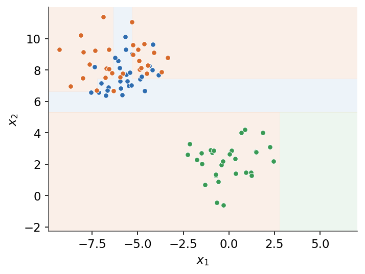	*A tree carves the input space into axis-aligned regions, each with a constant prediction.*
-	## 5.2 Random forests
+	## 7.2 Random forests
-	### 5.2.1 Bagging
+	### 7.2.1 Bagging
	Bagging (bootstrap aggregating) trains $B$ trees on $B$ bootstrap resamples of the data and averages them. The bagged predictor is defined as
@@ 84,7 84,7 @@
	A bootstrap sample draws $N$ examples with replacement from $N$ examples. The probability that a given example is never drawn is $(1-\tfrac1N)^N\to e^{-1}\approx0.37$, so about 37% of the data is left out of each tree. These are its out-of-bag (OOB) examples.
-	### 5.2.2 Variance of an average
+	### 7.2.2 Variance of an average
	If the $B$ trees each have variance $\sigma^2$ and pairwise correlation $\rho$, the variance of their average is
@@ 92,7 92,7 @@
	The second term vanishes as $B$ grows, but the first, $\rho\sigma^2$, does not. Reducing the correlation $\rho$ between trees is therefore the key lever, and that is what random forests target.
-	### 5.2.3 Random forests
+	### 7.2.3 Random forests
	A random forest is bagging plus feature subsampling: at each split only a random subset of $m_{\text{try}}$ features is considered as split candidates. The usual choices are
@@ 122,13 122,13 @@
	T3 --> AGG
	```
-	
+	
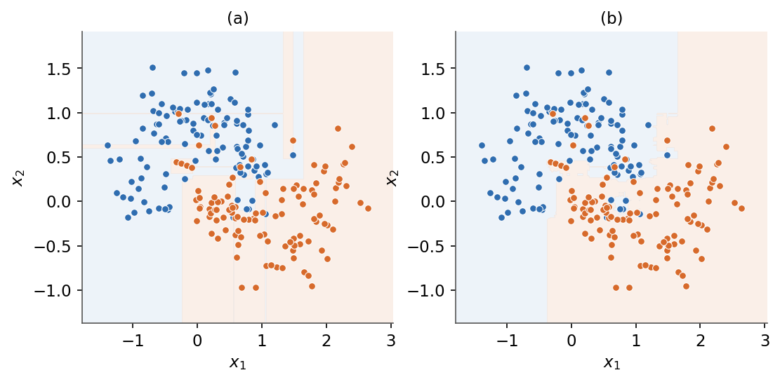	*(a) A single deep tree overfits with a jagged boundary. (b) A random forest averages many trees for a smoother boundary.*
-	## 5.3 Boosting
+	## 7.3 Boosting
-	### 5.3.1 Additive model
+	### 7.3.1 Additive model
	Boosting builds a predictor as a weighted sum of $T$ weak learners $h_t$ (typically shallow trees), fitted one at a time. The additive model is defined as
@@ 136,7 136,7 @@
	Each stage corrects the errors of the running sum, so the ensemble is built sequentially and reduces bias rather than variance.
-	### 5.3.2 AdaBoost
+	### 7.3.2 AdaBoost
	With labels $y\in\{-1,+1\}$, AdaBoost keeps example weights $w^{(i)}$ that concentrate on the currently misclassified points. At round $t$ the weak learner has weighted error $\varepsilon_t$, and its coefficient is defined as
@@ 148,7 148,7 @@
	and renormalized. Misclassified examples ($y^{(i)}h_t(x^{(i)})<0$) gain weight, so the next learner focuses on them.
-	### 5.3.3 Gradient boosting
+	### 7.3.3 Gradient boosting
	Gradient boosting generalizes the idea to any differentiable loss $L$. At stage $t$ it fits the next learner to the negative gradient of the loss evaluated at the current model, the pseudo-residual defined as
en/Machine Learning/05 Decision trees and ensemble methods/forest-vs-tree.png .. en/Machine Learning/07 Decision trees and ensemble methods/forest-vs-tree.png
en/Machine Learning/05 Decision trees and ensemble methods/tree-boundary.png .. en/Machine Learning/07 Decision trees and ensemble methods/tree-boundary.png
fr.md ..
@@ 1,9 1,10 @@
	# Cours ML & MLOps
-	Deux cours sur le machine learning et sa mise en production. Utilisez les drapeaux en haut de la
-	page pour changer de langue.
+	Trois cours sur le machine learning, le deep learning et la mise en production des modèles. Utilisez
+	les drapeaux en haut de la page pour changer de langue.
	## Cours
	- [Machine Learning](/fr/Machine%20Learning) : les fondements du ML, des données aux modèles.
+	- [Deep Learning](/fr/Deep%20Learning) : les réseaux de neurones, du perceptron aux transformeurs.
	- [MLOps](/fr/MLOps) : mettre les systèmes de ML en production et les maintenir.
/dev/null .. fr/Deep Learning.md
@@ 0,0 1,28 @@
+	# Deep Learning
+
+	Les réseaux de neurones, du simple perceptron aux transformeurs modernes : comment la profondeur, les bonnes fonctions d'activation et l'entraînement par gradient permettent à un modèle d'apprendre ses propres caractéristiques au lieu de les concevoir à la main.
+
+	**Prérequis :** le cours [Machine Learning](/fr/Machine%20Learning) (en particulier le perceptron dans [Modèles linéaires](/fr/Machine%20Learning/04%20Linear%20models)), Python de base, calcul différentiel et algèbre linéaire.
+
+	## Programme
+
+	1. [Introduction](/fr/Deep%20Learning/01%20Introduction)
+	2. [Perceptron multicouche](/fr/Deep%20Learning/02%20Multilayer%20perceptron)
+	3. [Fonctions d'activation](/fr/Deep%20Learning/03%20Activation%20functions)
+	4. [Fonctions de perte et couches de sortie](/fr/Deep%20Learning/04%20Loss%20functions%20and%20output%20layers)
+	5. [Rétropropagation](/fr/Deep%20Learning/05%20Backpropagation)
+	6. [Optimisation](/fr/Deep%20Learning/06%20Optimization)
+	7. [Initialisation et disparition du gradient](/fr/Deep%20Learning/07%20Initialization%20and%20vanishing%20gradients)
+	8. [Normalisation](/fr/Deep%20Learning/08%20Normalization)
+	9. [Régularisation et dropout](/fr/Deep%20Learning/09%20Regularization%20and%20dropout)
+	10. [Réseaux convolutifs](/fr/Deep%20Learning/10%20Convolutional%20networks)
+	11. [Architectures de CNN](/fr/Deep%20Learning/11%20CNN%20architectures)
+	12. [Plongements et apprentissage de représentations](/fr/Deep%20Learning/12%20Embeddings%20and%20representation%20learning)
+	13. [Réseaux récurrents](/fr/Deep%20Learning/13%20Recurrent%20networks)
+	14. [LSTM et GRU](/fr/Deep%20Learning/14%20LSTM%20and%20GRU)
+	15. [Attention](/fr/Deep%20Learning/15%20Attention)
+	16. [Transformeurs](/fr/Deep%20Learning/16%20Transformers)
+	17. [Le deep learning en pratique](/fr/Deep%20Learning/17%20Deep%20learning%20in%20practice)
+
+	---
+	[Machine Learning](/fr/Machine%20Learning) · [MLOps](/fr/MLOps) · [Accueil](/fr)
/dev/null .. fr/Deep Learning/01 Introduction.md
@@ 0,0 1,103 @@
+	# 1. Introduction
+
+	Ce cours prolonge directement le cours de Machine Learning, qui concluait la partie [Modèles linéaires](/fr/Machine%20Learning/04%20Linear%20models) sur une remarque clé : un perceptron est une unité unique, et empilé en couches il devient un réseau de neurones. Cette leçon rend ce pont explicite. Elle rappelle ce qu'une seule unité peut faire, montre la tâche concrète (XOR) où une unité unique échoue, et fixe la notation utilisée dans tout le reste du cours.
+
+	**Objectifs**
+	- Rappeler le perceptron comme une unité unique avec une activation en marche d'escalier et une frontière linéaire.
+	- Comprendre pourquoi une seule unité ne peut pas résoudre XOR, ce qui motive les couches cachées.
+	- Comprendre ce que signifie « profond » et pourquoi les couches cachées apprennent des caractéristiques.
+	- Adopter la notation à biais explicite, par couche, utilisée tout au long de ce cours.
+	- Lire un réseau comme une composition d'applications de couches, de l'entrée à la prédiction.
+
+	## 1.1 Le perceptron, rappel
+
+	Le perceptron du cours de Machine Learning est une unité de calcul unique. Il attribue un score à une entrée par une combinaison linéaire de ses caractéristiques et fait passer ce score par un seuil dur. Avec les paramètres $\theta$ et l'activation en marche d'escalier $g$, son hypothèse est :
+
+	$$\boxed{ h(x) = g(\theta^T x), \quad g(z) = \begin{cases} 1 & \text{if } z \ge 0 \\ 0 & \text{otherwise} \end{cases} }$$
+
+	L'équation $\theta^T x = 0$ est un hyperplan, donc le perceptron sépare l'espace d'entrée par une seule frontière plane. Les points d'un côté reçoivent l'étiquette $1$, les points de l'autre côté reçoivent l'étiquette $0$.
+
+	*Remarque :* la frontière est linéaire parce que le score $\theta^T x$ est linéaire en $x$. Le seuil ne fait que choisir un côté, il ne courbe pas la frontière.
+
+	## 1.2 Pourquoi une seule unité ne suffit pas
+
+	Une seule frontière linéaire ne peut résoudre que les problèmes dont les classes sont **linéairement séparables**, c'est-à-dire séparables par une unique coupe droite. Beaucoup de problèmes simples le sont, mais pas tous. Le contre-exemple classique est la fonction ou exclusif (XOR) de deux entrées binaires.
+
+	Les tables de vérité ci-dessous comparent AND, OR et XOR :
+
+	| $x_1$ | $x_2$ | AND | OR | XOR |
+	| --- | --- | --- | --- | --- |
+	| 0 | 0 | 0 | 0 | 0 |
+	| 0 | 1 | 0 | 1 | 1 |
+	| 1 | 0 | 0 | 1 | 1 |
+	| 1 | 1 | 1 | 1 | 0 |
+
+	
+
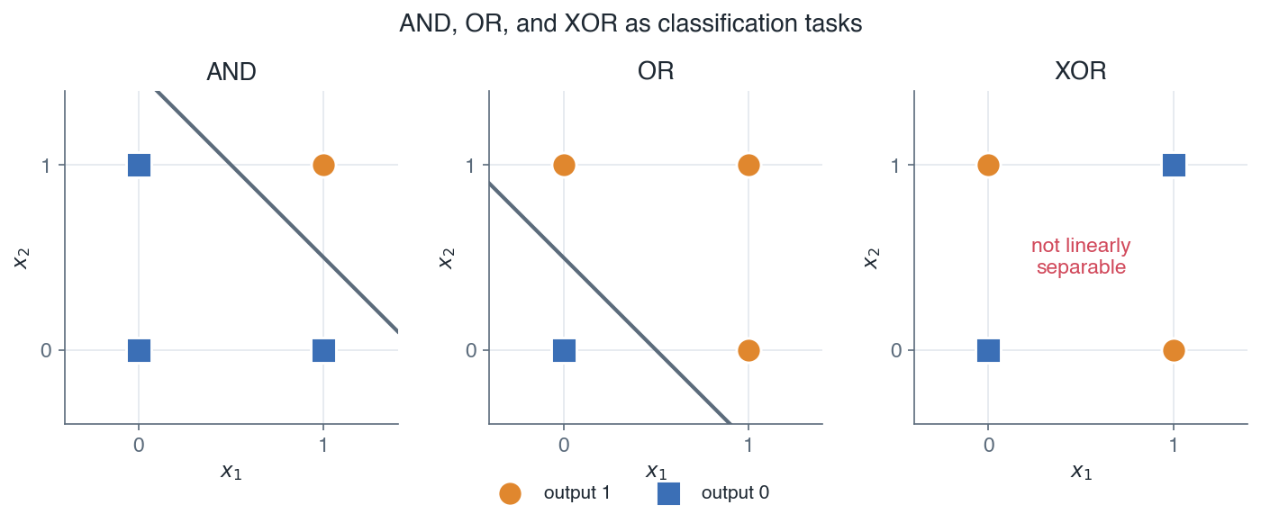+	*AND et OR sont séparables par une seule droite, mais XOR ne l'est pas, et c'est pourquoi une seule unité ne peut pas le résoudre.*
+
+	Pour AND et OR les deux classes de sortie peuvent être séparées par une seule droite, donc un perceptron les résout. Pour XOR les points positifs $(0,1)$ et $(1,0)$ sont sur une diagonale et les points négatifs $(0,0)$ et $(1,1)$ sur l'autre. Aucune droite unique ne peut les séparer.
+
+	*Remarque :* XOR n'est pas une curiosité isolée. Il montre que certains motifs sont intrinsèquement non linéaires, donc tout modèle construit à partir d'une seule frontière linéaire est fondamentalement limité. La solution consiste à combiner plusieurs unités.
+
+	Si l'on place une couche d'unités entre l'entrée et la sortie, les premières unités peuvent découper l'espace avec plusieurs frontières et une unité ultérieure peut combiner leurs sorties. Deux droites peuvent isoler le motif XOR là où une seule n'y parvient pas. Cette couche intermédiaire est une **couche cachée**, et c'est elle qui transforme une unité unique en réseau.
+
+	## 1.3 Des unités aux réseaux
+
+	Empiler des unités en couches, et des couches en un pipeline, donne un **réseau de neurones**. Un réseau est **profond** lorsqu'il possède plus d'une couche cachée entre l'entrée et la sortie. Chaque couche applique une application linéaire suivie d'une activation non linéaire, et les couches sont composées de sorte que la sortie de l'une alimente l'entrée de la suivante.
+
+	Le bénéfice est l'**apprentissage de représentations**. En apprentissage automatique classique, on conçoit les caractéristiques à la main, puis on les fournit à un modèle linéaire. Dans un réseau profond, les couches cachées apprennent leurs propres caractéristiques à partir de l'entrée brute : les premières couches capturent des motifs simples et les couches ultérieures les combinent en motifs plus abstraits. On spécifie l'architecture et l'objectif, et le réseau découvre les représentations intermédiaires par l'entraînement.
+
+	*Remarque :* empiler des applications linéaires seules reviendrait à une seule application linéaire, donc l'activation non linéaire $g$ entre les couches est essentielle. Sans elle, aucune profondeur n'ajouterait de puissance expressive. Les fonctions d'activation sont traitées dans les leçons suivantes.
+
+	## 1.4 Notation pour ce cours
+
+	Le cours de Machine Learning intégrait le biais dans le score avec la convention d'ordonnée à l'origine $x_0 = 1$, de sorte qu'un seul produit scalaire $\theta^T x$ portait le terme constant. Ce cours garde le biais **explicite** et utilise une matrice de poids distincte par couche. C'est la couture entre les deux cours : à partir d'ici, plus d'entrée augmentée et plus de biais intégré.
+
+	### 1.4.1 Une unité unique
+
+	Avec un biais explicite, une unité possède un vecteur de poids $w$ et un biais scalaire $b$. Son activation est :
+
+	$$\boxed{ a = g(w^T x + b) }$$
+
+	Le score $w^T x + b$ est la même fonction affine qu'auparavant, sauf que le biais $b$ est maintenant écrit explicitement au lieu d'être caché dans $\theta$.
+
+	### 1.4.2 Une couche et un réseau
+
+	Regroupons les unités de la couche $l$ dans une matrice de poids $W^{[l]}$ et un vecteur de biais $b^{[l]}$. La couche calcule une pré-activation $z^{[l]}$, puis une activation $a^{[l]}$ :
+
+	$$\boxed{ z^{[l]} = W^{[l]} a^{[l-1]} + b^{[l]}, \quad a^{[l]} = g^{[l]}(z^{[l]}) }$$
+
+	L'entrée alimente la première couche par $a^{[0]} = x$, et pour un réseau à $L$ couches la prédiction est la dernière activation :
+
+	$$\boxed{ a^{[0]} = x, \quad \hat{y} = a^{[L]} }$$
+
+	Ainsi le réseau est une composition d'applications de couches : $x = a^{[0]} \mapsto a^{[1]} \mapsto \cdots \mapsto a^{[L]} = \hat{y}$.
+
+	### 1.4.3 Table des symboles
+
+	| Symbole | Signification | Forme |
+	| --- | --- | --- |
+	| $L$ | nombre de couches | scalaire |
+	| $n_l$ | nombre d'unités dans la couche $l$ | scalaire |
+	| $W^{[l]}$ | matrice de poids de la couche $l$ | $n_l \times n_{l-1}$ |
+	| $b^{[l]}$ | vecteur de biais de la couche $l$ | $n_l$ |
+	| $z^{[l]}$ | pré-activation de la couche $l$ | $n_l$ |
+	| $a^{[l]}$ | activation de la couche $l$ | $n_l$ |
+	| $g^{[l]}$ | fonction d'activation de la couche $l$ | appliquée élément par élément |
+	| $\hat{y}$ | prédiction, égale à $a^{[L]}$ | $n_L$ |
+
+	*Remarque :* l'activation $g^{[l]}$ agit composante par composante, donc un produit élément par élément plus loin s'écrit avec le symbole de Hadamard $\odot$. L'exposant entre crochets, $[l]$, indexe la couche, ce n'est pas une puissance.
+
+	Le schéma suivant montre le plus petit réseau utile : une couche d'entrée, une couche cachée et une couche de sortie.
+
+	
+
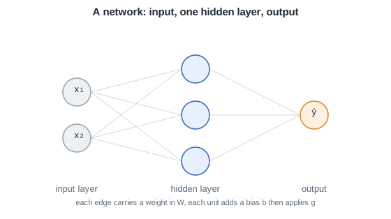+	*Un réseau de neurones : une couche d'entrée, une couche cachée et une sortie. Chaque arête porte un poids et chaque unité ajoute un biais puis applique une activation g.*
+
+	Chaque flèche porte un poids issu de $W^{[l]}$, et chaque unité cachée et de sortie ajoute son biais issu de $b^{[l]}$ avant d'appliquer son activation. Cette couche cachée à deux unités est exactement ce qui permet au réseau de résoudre XOR, la tâche qui mettait en échec une unité unique.
+
+	*La prochaine leçon formalise cette image sous la forme du perceptron multicouche, en écrivant la passe avant complète couche par couche et en choisissant les fonctions d'activation.*
+
+	---
+	Suivant : [Perceptron multicouche](/fr/Deep%20Learning/02%20Multilayer%20perceptron) · [Vue d'ensemble du cours](/fr/Deep%20Learning)
/dev/null .. fr/Deep Learning/01 Introduction/network-single-hidden.svg
@@ 0,0 1,1 @@
+	<svg xmlns="http://www.w3.org/2000/svg" viewBox="0 0 560 314" width="560" height="314" font-family="Helvetica, Arial, sans-serif"><defs><marker id="arrow" viewBox="0 0 10 10" refX="8.5" refY="5" markerWidth="7" markerHeight="7" orient="auto-start-reverse"><path d="M0 0L10 5L0 10z" fill="#1f2933"/></marker><marker id="arrowmuted" viewBox="0 0 10 10" refX="8.5" refY="5" markerWidth="7" markerHeight="7" orient="auto-start-reverse"><path d="M0 0L10 5L0 10z" fill="#5b6b7b"/></marker></defs><rect width="560" height="314" fill="#ffffff"/><text x="280.0" y="22.0" font-family="Helvetica, Arial, sans-serif" font-size="15" font-weight="600" fill="#1f2933" text-anchor="middle">A network: input, one hidden layer, output</text><line x1="130.0" y1="132.0" x2="260.0" y2="99.0" stroke="#c7d0d9" stroke-width="0.8"/><line x1="130.0" y1="132.0" x2="260.0" y2="165.0" stroke="#c7d0d9" stroke-width="0.8"/><line x1="130.0" y1="132.0" x2="260.0" y2="231.0" stroke="#c7d0d9" stroke-width="0.8"/><line x1="130.0" y1="198.0" x2="260.0" y2="99.0" stroke="#c7d0d9" stroke-width="0.8"/><line x1="130.0" y1="198.0" x2="260.0" y2="165.0" stroke="#c7d0d9" stroke-width="0.8"/><line x1="130.0" y1="198.0" x2="260.0" y2="231.0" stroke="#c7d0d9" stroke-width="0.8"/><line x1="300.0" y1="99.0" x2="430.0" y2="165.0" stroke="#c7d0d9" stroke-width="0.8"/><line x1="300.0" y1="165.0" x2="430.0" y2="165.0" stroke="#c7d0d9" stroke-width="0.8"/><line x1="300.0" y1="231.0" x2="430.0" y2="165.0" stroke="#c7d0d9" stroke-width="0.8"/><circle cx="110.0" cy="132.0" r="20.0" fill="#eef1f4" stroke="#9aa7b2" stroke-width="1.6"/><circle cx="110.0" cy="198.0" r="20.0" fill="#eef1f4" stroke="#9aa7b2" stroke-width="1.6"/><circle cx="280.0" cy="99.0" r="20.0" fill="#e8f0fe" stroke="#3b6fb6" stroke-width="1.6"/><circle cx="280.0" cy="165.0" r="20.0" fill="#e8f0fe" stroke="#3b6fb6" stroke-width="1.6"/><circle cx="280.0" cy="231.0" r="20.0" fill="#e8f0fe" stroke="#3b6fb6" stroke-width="1.6"/><circle cx="450.0" cy="165.0" r="20.0" fill="#fff1e0" stroke="#e0872e" stroke-width="1.6"/><text x="110.0" y="275.0" font-family="Helvetica, Arial, sans-serif" font-size="13" fill="#5b6b7b" text-anchor="middle">input layer</text><text x="280.0" y="275.0" font-family="Helvetica, Arial, sans-serif" font-size="13" fill="#5b6b7b" text-anchor="middle">hidden layer</text><text x="450.0" y="275.0" font-family="Helvetica, Arial, sans-serif" font-size="13" fill="#5b6b7b" text-anchor="middle">output</text><text x="110.0" y="132.0" font-family="Helvetica, Arial, sans-serif" font-size="13" fill="#1f2933" text-anchor="middle">x<tspan baseline-shift="sub" font-size="9px">1</tspan></text><text x="110.0" y="198.0" font-family="Helvetica, Arial, sans-serif" font-size="13" fill="#1f2933" text-anchor="middle">x<tspan baseline-shift="sub" font-size="9px">2</tspan></text><text x="450.0" y="165.0" font-family="Helvetica, Arial, sans-serif" font-size="13" fill="#1f2933" text-anchor="middle">ŷ</text><text x="280.0" y="294.0" font-family="Helvetica, Arial, sans-serif" font-size="11" fill="#5b6b7b" text-anchor="middle">each edge carries a weight in W, each unit adds a bias b then applies g</text></svg>
\	No newline at end of file
/dev/null .. fr/Deep Learning/01 Introduction/xor-problem.png
/dev/null .. fr/Deep Learning/02 Multilayer perceptron.md
@@ 0,0 1,100 @@
+	# 2. Perceptron multicouche
+
+	Un perceptron est une unité, $a = g(w^T x + b)$. Empilez plusieurs unités qui lisent la même entrée et vous obtenez une couche, empilez des couches et vous obtenez un perceptron multicouche (MLP). Ce module construit le MLP à partir d'unités, écrit la propagation avant pour un exemple et pour un mini-lot, suit les dimensions et le nombre de paramètres, et énonce le théorème d'approximation universelle.
+
+	**Objectifs**
+	- Construire une couche comme un empilement d'unités de type perceptron lisant une entrée partagée.
+	- Écrire la propagation avant pour un exemple avec des poids et un biais explicites par couche.
+	- Vectoriser la passe avant sur un mini-lot avec un biais diffusé.
+	- Suivre la dimension de chaque $W^{[l]}$ et $b^{[l]}$ et compter les paramètres.
+	- Énoncer le théorème d'approximation universelle et opposer la largeur à la profondeur.
+
+	## 2.1 D'une unité à une couche
+
+	### 2.1.1 Une seule unité
+
+	Une unité prend un vecteur d'entrée $x \in \mathbb{R}^{n_0}$, forme une somme pondérée avec un vecteur de poids $w$ et un biais scalaire $b$, puis applique une activation non linéaire $g$ :
+
+	$$\boxed{ a = g\left(w^T x + b\right) }$$
+
+	C'est le perceptron du cours précédent, sauf que le seuil dur est maintenant une activation lisse comme la sigmoïde ou la ReLU. L'activation est nommée ici et définie complètement dans la [leçon suivante](/fr/Deep%20Learning/03%20Activation%20functions).
+
+	### 2.1.2 Une couche d'unités
+
+	Placez maintenant $n_1$ unités côte à côte, lisant toutes la même entrée $x$. L'unité $i$ possède son propre vecteur de poids $w_i$ et son biais $b_i$, produisant $a_i = g(w_i^T x + b_i)$. Rassemblez les vecteurs de poids comme les lignes d'une matrice $W^{[1]}$ et les biais dans un vecteur $b^{[1]}$ :
+
+	$$\boxed{ W^{[1]} = \begin{bmatrix} w_1^{T} \\ \vdots \\ w_{n_1}^{T} \end{bmatrix}, \quad b^{[1]} = \begin{bmatrix} b_1 \\ \vdots \\ b_{n_1} \end{bmatrix} }$$
+
+	La couche entière calcule alors un vecteur de pré-activation et un vecteur d'activation en une seule expression matricielle, $z^{[1]} = W^{[1]} x + b^{[1]}$ et $a^{[1]} = g^{[1]}(z^{[1]})$, où $g^{[1]}$ est appliquée élément par élément.
+
+	*Remarque :* les lignes de $W^{[1]}$ sont exactement les vecteurs de poids des unités individuelles, donc une couche n'est que de nombreuses unités regroupées dans une seule matrice. Le biais reste explicite ici : contrairement au cours de Machine Learning, qui intégrait l'ordonnée à l'origine dans $\theta$ via l'entrée augmentée $x_0 = 1$, ce cours conserve $b^{[l]}$ comme son propre vecteur.
+
+	## 2.2 Propagation avant
+
+	L'empilement de $L$ telles couches donne le MLP. La couche $l$ lit l'activation de la couche inférieure, $a^{[l-1]}$, et produit $a^{[l]}$. L'entrée est $a^{[0]} = x$ et la prédiction est la sortie de la dernière couche.
+
+	### 2.2.1 Un exemple
+
+	Pour $l = 1, \dots, L$ :
+
+	$$\boxed{ a^{[0]} = x, \quad z^{[l]} = W^{[l]} a^{[l-1]} + b^{[l]}, \quad a^{[l]} = g^{[l]}\!\left(z^{[l]}\right), \quad \hat{y} = a^{[L]} }$$
+
+	Chaque couche peut utiliser sa propre activation $g^{[l]}$ : les couches cachées utilisent typiquement la ReLU, tandis que la couche de sortie utilise la sigmoïde ou le softmax pour la classification et l'identité pour la régression.
+
+	*Remarque :* la composition $\hat{y} = g^{[L]}(W^{[L]} g^{[L-1]}(\cdots g^{[1]}(W^{[1]} x + b^{[1]}) \cdots) + b^{[L]})$ est ce qui rend le réseau expressif. Sans les $g^{[l]}$ non linéaires, l'empilement entier s'effondrerait en une seule application linéaire $W x + b$.
+
+	### 2.2.2 Vectorisation sur un mini-lot
+
+	L'entraînement s'exécute sur des lots, pas sur des exemples isolés. Placez $m$ exemples comme les colonnes d'une matrice, de sorte que $A^{[0]} = X \in \mathbb{R}^{n_0 \times m}$, et la passe avant devient un produit matriciel avec le biais diffusé sur toutes les colonnes :
+
+	$$\boxed{ Z^{[l]} = W^{[l]} A^{[l-1]} + b^{[l]}, \quad A^{[l]} = g^{[l]}\!\left(Z^{[l]}\right) }$$
+
+	Ici $Z^{[l]}$ et $A^{[l]}$ ont pour dimension $n_l \times m$, une colonne par exemple. Le biais $b^{[l]} \in \mathbb{R}^{n_l}$ est ajouté à chaque colonne, une opération connue sous le nom de diffusion (broadcasting).
+
+	*Remarque :* le seul changement par rapport à la forme à un exemple est que le vecteur $a^{[l-1]}$ devient la matrice $A^{[l-1]}$. Traiter un lot en une seule multiplication matricielle est ce qui permet à un GPU d'exécuter la passe efficacement.
+
+	## 2.3 Dimensions et nombre de paramètres
+
+	Les dimensions découlent d'une seule règle : pour calculer $z^{[l]} = W^{[l]} a^{[l-1]} + b^{[l]}$, la matrice $W^{[l]}$ doit envoyer un vecteur de dimension $n_{l-1}$ vers un vecteur de dimension $n_l$.
+
+	$$\boxed{ W^{[l]} \in \mathbb{R}^{n_l \times n_{l-1}}, \quad b^{[l]} \in \mathbb{R}^{n_l} }$$
+
+	La couche $l$ contient donc $n_l \, n_{l-1}$ poids plus $n_l$ biais. Considérons un petit réseau avec $n_0 = 4$ entrées, deux couches cachées de $5$ et $3$ unités, et une seule unité de sortie.
+
+	| Couche $l$ | Dimension de $W^{[l]}$ | Dimension de $b^{[l]}$ | Paramètres |
+	| --- | --- | --- | --- |
+	| 1 | $5 \times 4$ | $5$ | $25$ |
+	| 2 | $3 \times 5$ | $3$ | $18$ |
+	| 3 | $1 \times 3$ | $1$ | $4$ |
+	| Total | | | $47$ |
+
+	*Remarque :* la couche d'entrée ne contient aucun paramètre, elle n'est que les données $a^{[0]} = x$. Quand on compte les couches, on compte celles qui portent des poids, donc ce réseau a $L = 3$.
+
+	## 2.4 Un réseau multicouche
+
+	Le diagramme ci-dessous montre le même réseau $4$-$5$-$3$-$1$ sous forme d'un flux d'activations. Chaque groupe de flèches est une matrice de poids complète, et chaque boîte applique son activation à la pré-activation.
+
+	
+
+	*Un perceptron multicouche : chaque couche calcule z = W a + b puis a = g(z), composant l'entrée a0 en la prédiction aL.*
+
+	L'information circule strictement de gauche à droite pendant la passe avant, c'est pourquoi il s'agit d'un réseau à propagation avant (feedforward). Rien ne boucle en arrière. La direction inverse, utilisée pour calculer les gradients, fait l'objet d'une leçon ultérieure.
+
+	## 2.5 Approximation universelle
+
+	Quelle est l'expressivité d'un MLP ? Le théorème d'approximation universelle apporte une réponse forte. Soit $f$ une fonction continue quelconque sur un compact $K \subset \mathbb{R}^{n_0}$, et soit $\varepsilon > 0$. Alors il existe un réseau avec une seule couche cachée de largeur finie, utilisant une activation non linéaire appropriée, dont la sortie $F$ vérifie :
+
+	$$\boxed{ \sup_{x \in K} \left| F(x) - f(x) \right| < \varepsilon }$$
+
+	Autrement dit, une seule couche cachée avec suffisamment d'unités peut approcher n'importe quelle fonction continue sur une région bornée avec la précision souhaitée $\varepsilon$. C'est un résultat d'existence, pas une recette : il garantit que de tels poids existent, mais ne dit rien sur le nombre d'unités nécessaires ni sur la manière de les trouver.
+
+	*Remarque :* le piège est la largeur. Atteindre une cible avec une précision $\varepsilon$ avec une seule couche cachée peut exiger un nombre énorme d'unités, croissant rapidement à mesure que $\varepsilon$ diminue. La profondeur est généralement bien plus efficace en paramètres : empiler plusieurs couches étroites peut représenter des fonctions qu'une seule couche nécessiterait un nombre exponentiel d'unités pour égaler. Cette efficacité de la profondeur sur la largeur est la raison pratique pour laquelle le domaine s'appelle l'apprentissage profond (deep learning).
+
+	
+
+	*Un réseau avec une seule couche cachée approche une fonction cible en sommant de nombreuses unités activées simples.*
+
+	*Le réseau n'est défini qu'une fois les activations $g^{[l]}$ fixées. La leçon suivante les définit, sigmoïde, tanh, ReLU et ses variantes, et explique comment chacune façonne l'apprentissage.*
+
+	---
+	Suivant : [Fonctions d'activation](/fr/Deep%20Learning/03%20Activation%20functions) · [Vue d'ensemble du cours](/fr/Deep%20Learning)
/dev/null .. fr/Deep Learning/02 Multilayer perceptron/mlp-forward.svg
@@ 0,0 1,1 @@
+	<svg xmlns="http://www.w3.org/2000/svg" viewBox="0 0 760 392" width="760" height="392" font-family="Helvetica, Arial, sans-serif"><defs><marker id="arrow" viewBox="0 0 10 10" refX="8.5" refY="5" markerWidth="7" markerHeight="7" orient="auto-start-reverse"><path d="M0 0L10 5L0 10z" fill="#1f2933"/></marker><marker id="arrowmuted" viewBox="0 0 10 10" refX="8.5" refY="5" markerWidth="7" markerHeight="7" orient="auto-start-reverse"><path d="M0 0L10 5L0 10z" fill="#5b6b7b"/></marker></defs><rect width="760" height="392" fill="#ffffff"/><text x="380.0" y="22.0" font-family="Helvetica, Arial, sans-serif" font-size="15" font-weight="600" fill="#1f2933" text-anchor="middle">Forward propagation through a 4-5-3-1 network</text><line x1="136.0" y1="125.0" x2="274.0" y2="100.0" stroke="#c7d0d9" stroke-width="0.8"/><line x1="136.0" y1="125.0" x2="274.0" y2="150.0" stroke="#c7d0d9" stroke-width="0.8"/><line x1="136.0" y1="125.0" x2="274.0" y2="200.0" stroke="#c7d0d9" stroke-width="0.8"/><line x1="136.0" y1="125.0" x2="274.0" y2="250.0" stroke="#c7d0d9" stroke-width="0.8"/><line x1="136.0" y1="125.0" x2="274.0" y2="300.0" stroke="#c7d0d9" stroke-width="0.8"/><line x1="136.0" y1="175.0" x2="274.0" y2="100.0" stroke="#c7d0d9" stroke-width="0.8"/><line x1="136.0" y1="175.0" x2="274.0" y2="150.0" stroke="#c7d0d9" stroke-width="0.8"/><line x1="136.0" y1="175.0" x2="274.0" y2="200.0" stroke="#c7d0d9" stroke-width="0.8"/><line x1="136.0" y1="175.0" x2="274.0" y2="250.0" stroke="#c7d0d9" stroke-width="0.8"/><line x1="136.0" y1="175.0" x2="274.0" y2="300.0" stroke="#c7d0d9" stroke-width="0.8"/><line x1="136.0" y1="225.0" x2="274.0" y2="100.0" stroke="#c7d0d9" stroke-width="0.8"/><line x1="136.0" y1="225.0" x2="274.0" y2="150.0" stroke="#c7d0d9" stroke-width="0.8"/><line x1="136.0" y1="225.0" x2="274.0" y2="200.0" stroke="#c7d0d9" stroke-width="0.8"/><line x1="136.0" y1="225.0" x2="274.0" y2="250.0" stroke="#c7d0d9" stroke-width="0.8"/><line x1="136.0" y1="225.0" x2="274.0" y2="300.0" stroke="#c7d0d9" stroke-width="0.8"/><line x1="136.0" y1="275.0" x2="274.0" y2="100.0" stroke="#c7d0d9" stroke-width="0.8"/><line x1="136.0" y1="275.0" x2="274.0" y2="150.0" stroke="#c7d0d9" stroke-width="0.8"/><line x1="136.0" y1="275.0" x2="274.0" y2="200.0" stroke="#c7d0d9" stroke-width="0.8"/><line x1="136.0" y1="275.0" x2="274.0" y2="250.0" stroke="#c7d0d9" stroke-width="0.8"/><line x1="136.0" y1="275.0" x2="274.0" y2="300.0" stroke="#c7d0d9" stroke-width="0.8"/><line x1="306.0" y1="100.0" x2="444.0" y2="150.0" stroke="#c7d0d9" stroke-width="0.8"/><line x1="306.0" y1="100.0" x2="444.0" y2="200.0" stroke="#c7d0d9" stroke-width="0.8"/><line x1="306.0" y1="100.0" x2="444.0" y2="250.0" stroke="#c7d0d9" stroke-width="0.8"/><line x1="306.0" y1="150.0" x2="444.0" y2="150.0" stroke="#c7d0d9" stroke-width="0.8"/><line x1="306.0" y1="150.0" x2="444.0" y2="200.0" stroke="#c7d0d9" stroke-width="0.8"/><line x1="306.0" y1="150.0" x2="444.0" y2="250.0" stroke="#c7d0d9" stroke-width="0.8"/><line x1="306.0" y1="200.0" x2="444.0" y2="150.0" stroke="#c7d0d9" stroke-width="0.8"/><line x1="306.0" y1="200.0" x2="444.0" y2="200.0" stroke="#c7d0d9" stroke-width="0.8"/><line x1="306.0" y1="200.0" x2="444.0" y2="250.0" stroke="#c7d0d9" stroke-width="0.8"/><line x1="306.0" y1="250.0" x2="444.0" y2="150.0" stroke="#c7d0d9" stroke-width="0.8"/><line x1="306.0" y1="250.0" x2="444.0" y2="200.0" stroke="#c7d0d9" stroke-width="0.8"/><line x1="306.0" y1="250.0" x2="444.0" y2="250.0" stroke="#c7d0d9" stroke-width="0.8"/><line x1="306.0" y1="300.0" x2="444.0" y2="150.0" stroke="#c7d0d9" stroke-width="0.8"/><line x1="306.0" y1="300.0" x2="444.0" y2="200.0" stroke="#c7d0d9" stroke-width="0.8"/><line x1="306.0" y1="300.0" x2="444.0" y2="250.0" stroke="#c7d0d9" stroke-width="0.8"/><line x1="476.0" y1="150.0" x2="614.0" y2="200.0" stroke="#c7d0d9" stroke-width="0.8"/><line x1="476.0" y1="200.0" x2="614.0" y2="200.0" stroke="#c7d0d9" stroke-width="0.8"/><line x1="476.0" y1="250.0" x2="614.0" y2="200.0" stroke="#c7d0d9" stroke-width="0.8"/><circle cx="120.0" cy="125.0" r="16.0" fill="#eef1f4" stroke="#9aa7b2" stroke-width="1.6"/><circle cx="120.0" cy="175.0" r="16.0" fill="#eef1f4" stroke="#9aa7b2" stroke-width="1.6"/><circle cx="120.0" cy="225.0" r="16.0" fill="#eef1f4" stroke="#9aa7b2" stroke-width="1.6"/><circle cx="120.0" cy="275.0" r="16.0" fill="#eef1f4" stroke="#9aa7b2" stroke-width="1.6"/><circle cx="290.0" cy="100.0" r="16.0" fill="#e8f0fe" stroke="#3b6fb6" stroke-width="1.6"/><circle cx="290.0" cy="150.0" r="16.0" fill="#e8f0fe" stroke="#3b6fb6" stroke-width="1.6"/><circle cx="290.0" cy="200.0" r="16.0" fill="#e8f0fe" stroke="#3b6fb6" stroke-width="1.6"/><circle cx="290.0" cy="250.0" r="16.0" fill="#e8f0fe" stroke="#3b6fb6" stroke-width="1.6"/><circle cx="290.0" cy="300.0" r="16.0" fill="#e8f0fe" stroke="#3b6fb6" stroke-width="1.6"/><circle cx="460.0" cy="150.0" r="16.0" fill="#e8f0fe" stroke="#3b6fb6" stroke-width="1.6"/><circle cx="460.0" cy="200.0" r="16.0" fill="#e8f0fe" stroke="#3b6fb6" stroke-width="1.6"/><circle cx="460.0" cy="250.0" r="16.0" fill="#e8f0fe" stroke="#3b6fb6" stroke-width="1.6"/><circle cx="630.0" cy="200.0" r="16.0" fill="#fff1e0" stroke="#e0872e" stroke-width="1.6"/><text x="120.0" y="355.0" font-family="Helvetica, Arial, sans-serif" font-size="13" fill="#5b6b7b" text-anchor="middle">a<tspan baseline-shift="sub" font-size="9px">0</tspan> (input)</text><text x="290.0" y="355.0" font-family="Helvetica, Arial, sans-serif" font-size="13" fill="#5b6b7b" text-anchor="middle">a<tspan baseline-shift="sub" font-size="9px">1</tspan></text><text x="460.0" y="355.0" font-family="Helvetica, Arial, sans-serif" font-size="13" fill="#5b6b7b" text-anchor="middle">a<tspan baseline-shift="sub" font-size="9px">2</tspan></text><text x="630.0" y="355.0" font-family="Helvetica, Arial, sans-serif" font-size="13" fill="#5b6b7b" text-anchor="middle">a<tspan baseline-shift="sub" font-size="9px">3</tspan> = ŷ</text><text x="205.0" y="90.0" font-family="Helvetica, Arial, sans-serif" font-size="12" fill="#5b6b7b" text-anchor="middle">W a + b</text><text x="380.0" y="372.0" font-family="Helvetica, Arial, sans-serif" font-size="11" fill="#5b6b7b" text-anchor="middle">each box computes z = W a + b then a = g(z), information flows left to right</text></svg>
\	No newline at end of file
/dev/null .. fr/Deep Learning/02 Multilayer perceptron/universal-approximation.png
/dev/null .. fr/Deep Learning/03 Activation functions.md
@@ 0,0 1,103 @@
+	# 3. Fonctions d'activation
+
+	Chaque couche calcule une pré-activation $z^{[l]} = W^{[l]} a^{[l-1]} + b^{[l]}$ puis une activation $a^{[l]} = g^{[l]}(z^{[l]})$. Le choix de la non-linéarité $g^{[l]}$ est ce qui rend la profondeur utile. Cette leçon explique pourquoi une fonction $g$ non linéaire est nécessaire, passe en revue les familles sigmoïde, tanh et ReLU, présente la softmax utilisée en sortie et donne des conseils pratiques sur l'activation à choisir.
+
+	**Objectifs**
+	- Montrer qu'un empilement de couches purement linéaires se réduit à une seule application linéaire.
+	- Définir la sigmoïde et la tanh, dériver leurs dérivées et expliquer la saturation.
+	- Passer en revue la famille ReLU (ReLU, leaky ReLU, PReLU, ELU, GELU) et le problème des unités mortes.
+	- Définir la softmax et la placer en sortie plutôt que dans les couches cachées.
+	- Donner une règle empirique simple pour choisir une activation par couche.
+
+	## 3.1 Pourquoi la non-linéarité est nécessaire
+
+	Supposons que chaque activation soit l'identité, $g^{[l]}(z) = z$. Alors chaque couche se réduit à $a^{[l]} = W^{[l]} a^{[l-1]} + b^{[l]}$, et composer deux d'entre elles donne $W^{[2]}(W^{[1]} x + b^{[1]}) + b^{[2]} = (W^{[2]} W^{[1]}) x + (W^{[2]} b^{[1]} + b^{[2]})$. C'est de nouveau de la forme $W x + b$. Par récurrence, l'ensemble du réseau à $L$ couches se réduit à une seule application affine :
+
+	$$\boxed{ g^{[l]} = \text{identity} \;\Rightarrow\; \hat{y} = W' x + b' }$$
+
+	avec $W' = W^{[L]} \cdots W^{[1]}$ et $b'$ le biais accumulé. Peu importe le nombre de couches linéaires empilées, le modèle ne peut ajuster qu'une fonction linéaire, donc la profondeur supplémentaire n'apporte rien. Une fonction $g$ non linéaire entre les couches est précisément ce qui brise cet effondrement et permet au réseau de représenter des frontières de décision courbes et des régressions non linéaires.
+
+	*Remarque :* le biais est conservé ici de façon explicite sous la forme $b^{[l]}$, contrairement au cours de Machine Learning où l'ordonnée à l'origine était intégrée dans $\theta^T x$ via l'entrée augmentée $x_0 = 1$. Dans ce cours de Deep Learning, chaque couche possède sa propre matrice de poids $W^{[l]}$ et son propre vecteur de biais $b^{[l]}$.
+
+	## 3.2 Sigmoïde et tanh
+
+	
+
+	*Fonctions d'activation courantes : la sigmoïde et la tanh, bornées, saturent dans leurs queues, tandis que ReLU et ses variantes restent linéaires pour les entrées positives.*
+
+	### 3.2.1 Sigmoïde
+
+	La sigmoïde écrase n'importe quelle pré-activation réelle dans l'intervalle ouvert $(0, 1)$ :
+
+	$$\boxed{ \sigma(z) = \frac{1}{1 + e^{-z}} \in (0, 1) }$$
+
+	Sa dérivée admet la forme close pratique ci-dessous, qui réutilise la valeur avant $\sigma(z)$ déjà calculée :
+
+	$$\boxed{ \sigma'(z) = \sigma(z)\left(1 - \sigma(z)\right) }$$
+
+	### 3.2.2 Tanh
+
+	La tangente hyperbolique est une sigmoïde remise à l'échelle et centrée en zéro, dont la sortie est dans $(-1, 1)$. Sa dérivée s'exprime elle aussi à partir de la valeur avant :
+
+	$$\boxed{ \tanh'(z) = 1 - \tanh(z)^2 }$$
+
+	*Remarque :* $\tanh$ est centrée en zéro alors que $\sigma$ ne l'est pas, si bien que $\tanh$ s'entraîne souvent un peu mieux comme activation cachée. Les deux sont reliées par $\tanh(z) = 2\sigma(2z) - 1$.
+
+	### 3.2.3 Saturation
+
+	Les deux courbes s'aplatissent dans leurs queues. Pour de grandes valeurs de $|z|$, la sortie est proche d'une constante ($0$ ou $1$ pour $\sigma$, $\pm 1$ pour $\tanh$), donc la dérivée est proche de zéro : $\sigma'(z) \to 0$ et $\tanh'(z) \to 0$. Une unité située dans cette région plate est dite saturée, et elle ne transmet presque aucun gradient vers l'arrière. Lorsque de nombreux facteurs de ce type se multiplient à travers un empilement profond, le gradient tend vers zéro : c'est le problème de disparition du gradient revu dans [Initialisation et disparition du gradient](/fr/Deep%20Learning/07%20Initialization%20and%20vanishing%20gradients).
+
+	
+
+	*Dérivées des activations : les gradients de la sigmoïde et de la tanh disparaissent dans les queues, tandis que le gradient de ReLU vaut 1 partout où l'unité est active.*
+
+	## 3.3 La famille ReLU
+
+	L'unité linéaire rectifiée conserve la partie positive de son entrée et annule le reste :
+
+	$$\boxed{ \text{ReLU}(z) = \max(0, z) }$$
+
+	Sa dérivée vaut $1$ pour $z > 0$ et $0$ pour $z < 0$ (non définie en $z = 0$, prise égale à $0$ ou $1$ par convention). ReLU ne sature pas du côté positif, elle y maintient donc un gradient sain, ce qui explique en grande partie pourquoi elle est devenue l'activation cachée par défaut. Le prix à payer est le problème des unités mortes : si la pré-activation d'une unité est toujours négative sur l'ensemble des données, son gradient est toujours nul et elle cesse complètement d'apprendre. Les variantes ci-dessous sacrifient un peu de simplicité pour adoucir cette défaillance ou lisser le point anguleux à l'origine.
+
+	| nom | formule | dérivée | meurt / sature ? |
+	| --- | --- | --- | --- |
+	| ReLU | $\max(0, z)$ | $1$ if $z>0$ else $0$ | peut mourir (gradient nul pour $z<0$) |
+	| Leaky ReLU | $\max(\alpha z, z)$, $\alpha \approx 0.01$ | $1$ if $z>0$ else $\alpha$ | meurt rarement (petite pente négative) |
+	| PReLU | $\max(\alpha z, z)$, $\alpha$ learned | $1$ if $z>0$ else $\alpha$ | meurt rarement ($\alpha$ appris par canal) |
+	| ELU | $z$ if $z>0$ else $\alpha(e^z - 1)$ | $1$ if $z>0$ else $\alpha e^z$ | sature doucement pour $z\to-\infty$ |
+	| GELU | $z\,\Phi(z)$, $\Phi$ the normal CDF | lisse, proche de $1$ pour de grands $z$ | lisse, pas de mort brutale |
+
+	*Remarque :* leaky ReLU et PReLU ajoutent une petite pente $\alpha$ du côté négatif afin qu'une unité ne soit jamais complètement éteinte. GELU pondère l'entrée par la probabilité $\Phi(z)$ qu'une loi normale standard soit inférieure à $z$, ce qui donne une courbe lisse se comportant comme ReLU pour de grandes valeurs de $|z|$. C'est le choix standard à l'intérieur des Transformers.
+
+	## 3.4 Softmax pour les sorties multiclasses
+
+	Pour une classification à $K$ classes, la couche finale produit un vecteur $z \in \mathbb{R}^K$ de scores, et la softmax le transforme en une distribution de probabilité sur les classes :
+
+	$$\boxed{ \text{softmax}(z)_k = \frac{e^{z_k}}{\sum_{j=1}^{K} e^{z_j}} }$$
+
+	Chaque composante appartient à $(0, 1)$ et les composantes somment à $1$, si bien que $\text{softmax}(z)_k$ se lit comme la probabilité prédite de la classe $k$. Le plus grand score devient la classe la plus probable.
+
+	*Remarque :* la softmax a sa place dans la couche de sortie, pas dans une couche cachée. Elle couple chaque unité par le dénominateur partagé (une normalisation sur tout le vecteur), ce qui est exactement ce dont une sortie probabiliste a besoin mais ne constitue pas une non-linéarité cachée utile par unité. Pour une sortie unique ($K = 1$ contre son complément), la softmax se réduit à la sigmoïde. L'association de la softmax avec sa fonction de perte fait l'objet de [Fonctions de perte et couches de sortie](/fr/Deep%20Learning/04%20Loss%20functions%20and%20output%20layers).
+
+	## 3.5 Choisir une activation
+
+	Un bon choix par défaut : utiliser ReLU ou GELU dans les couches cachées, et choisir l'activation de sortie selon la tâche. Le schéma et le tableau ci-dessous résument la décision.
+
+	
+
+	*Choisir une activation : ReLU ou GELU pour les couches cachées, et une activation de sortie adaptée à la tâche.*
+
+	| couche / tâche | activation recommandée | raison |
+	| --- | --- | --- |
+	| cachée (par défaut) | ReLU ou GELU | pas de saturation du côté positif, peu coûteuse, entraînement rapide |
+	| cachée (unités mortes) | leaky ReLU ou ELU | conserve un gradient non nul pour $z < 0$ |
+	| sortie, régression | identité (aucune) | la prédiction est une valeur réelle non bornée |
+	| sortie, binaire | sigmoïde | transforme le score en une probabilité dans $(0, 1)$ |
+	| sortie, multiclasse | softmax | transforme les scores en une distribution sur les classes |
+
+	*Remarque :* la sigmoïde et la tanh sont aujourd'hui rarement utilisées comme activations cachées dans les réseaux profonds à propagation avant, précisément à cause de la saturation vue à la Section 3.2.3. Elles subsistent en sortie (sigmoïde) et à l'intérieur des unités récurrentes à portes, où leur plage bornée est justement recherchée.
+
+	*Une fois les non-linéarités par couche fixées, la prochaine leçon associe l'activation de sortie à une fonction de perte adaptée afin que le réseau ait quelque chose à minimiser.*
+
+	---
+	Suivant : [Fonctions de perte et couches de sortie](/fr/Deep%20Learning/04%20Loss%20functions%20and%20output%20layers) · [Vue d'ensemble du cours](/fr/Deep%20Learning)
/dev/null .. fr/Deep Learning/03 Activation functions/activation-choice.svg
@@ 0,0 1,1 @@
+	<svg xmlns="http://www.w3.org/2000/svg" viewBox="0 0 920 542" width="920" height="542" font-family="Helvetica, Arial, sans-serif"><defs><marker id="arrow" viewBox="0 0 10 10" refX="8.5" refY="5" markerWidth="7" markerHeight="7" orient="auto-start-reverse"><path d="M0 0L10 5L0 10z" fill="#1f2933"/></marker><marker id="arrowmuted" viewBox="0 0 10 10" refX="8.5" refY="5" markerWidth="7" markerHeight="7" orient="auto-start-reverse"><path d="M0 0L10 5L0 10z" fill="#5b6b7b"/></marker></defs><rect width="920" height="542" fill="#ffffff"/><text x="460.0" y="22.0" font-family="Helvetica, Arial, sans-serif" font-size="15" font-weight="600" fill="#1f2933" text-anchor="middle">Choosing an activation</text><rect x="340.0" y="44.0" width="200.0" height="46.0" rx="8" fill="#eef1f4" stroke="#9aa7b2" stroke-width="1.6"/><text x="440.0" y="71.4" font-family="Helvetica, Arial, sans-serif" font-size="13" fill="#1f2933" text-anchor="middle">which layer?</text><rect x="340.0" y="124.0" width="200.0" height="46.0" rx="8" fill="#e4f5f4" stroke="#2a9d9a" stroke-width="1.6"/><text x="440.0" y="151.4" font-family="Helvetica, Arial, sans-serif" font-size="13" fill="#1f2933" text-anchor="middle">hidden or output?</text><line x1="440.0" y1="90.0" x2="440.0" y2="124.0" stroke="#1f2933" stroke-width="1.7" marker-end="url(#arrow)"/><rect x="60.0" y="214.0" width="200.0" height="46.0" rx="8" fill="#e8f0fe" stroke="#3b6fb6" stroke-width="1.6"/><text x="160.0" y="241.4" font-family="Helvetica, Arial, sans-serif" font-size="13" fill="#1f2933" text-anchor="middle">ReLU or GELU default</text><line x1="360.0" y1="170.0" x2="190.0" y2="214.0" stroke="#1f2933" stroke-width="1.7" marker-end="url(#arrow)"/><text x="275.0" y="187.0" font-family="Helvetica, Arial, sans-serif" font-size="11" fill="#5b6b7b" text-anchor="middle">hidden</text><rect x="60.0" y="298.0" width="200.0" height="46.0" rx="8" fill="#e4f5f4" stroke="#2a9d9a" stroke-width="1.6"/><text x="160.0" y="325.4" font-family="Helvetica, Arial, sans-serif" font-size="13" fill="#1f2933" text-anchor="middle">units dying?</text><line x1="160.0" y1="260.0" x2="160.0" y2="298.0" stroke="#1f2933" stroke-width="1.7" marker-end="url(#arrow)"/><rect x="20.0" y="392.0" width="190.0" height="46.0" rx="8" fill="#fff1e0" stroke="#e0872e" stroke-width="1.6"/><text x="115.0" y="419.4" font-family="Helvetica, Arial, sans-serif" font-size="13" fill="#1f2933" text-anchor="middle">leaky ReLU or ELU</text><line x1="120.0" y1="344.0" x2="90.0" y2="392.0" stroke="#1f2933" stroke-width="1.7" marker-end="url(#arrow)"/><text x="105.0" y="363.0" font-family="Helvetica, Arial, sans-serif" font-size="11" fill="#5b6b7b" text-anchor="middle">yes</text><rect x="240.0" y="392.0" width="190.0" height="46.0" rx="8" fill="#e7f5ea" stroke="#38a05a" stroke-width="1.6"/><text x="335.0" y="419.4" font-family="Helvetica, Arial, sans-serif" font-size="13" fill="#1f2933" text-anchor="middle">keep ReLU or GELU</text><line x1="200.0" y1="344.0" x2="300.0" y2="392.0" stroke="#1f2933" stroke-width="1.7" marker-end="url(#arrow)"/><text x="250.0" y="363.0" font-family="Helvetica, Arial, sans-serif" font-size="11" fill="#5b6b7b" text-anchor="middle">no</text><rect x="520.0" y="214.0" width="200.0" height="46.0" rx="8" fill="#e4f5f4" stroke="#2a9d9a" stroke-width="1.6"/><text x="620.0" y="241.4" font-family="Helvetica, Arial, sans-serif" font-size="13" fill="#1f2933" text-anchor="middle">task type?</text><line x1="520.0" y1="170.0" x2="620.0" y2="214.0" stroke="#1f2933" stroke-width="1.7" marker-end="url(#arrow)"/><text x="570.0" y="187.0" font-family="Helvetica, Arial, sans-serif" font-size="11" fill="#5b6b7b" text-anchor="middle">output</text><line x1="640.0" y1="260.0" x2="640.0" y2="479.0" stroke="#1f2933" stroke-width="1.6"/><rect x="680.0" y="300.0" width="190.0" height="46.0" rx="8" fill="#e7f5ea" stroke="#38a05a" stroke-width="1.6"/><text x="775.0" y="327.4" font-family="Helvetica, Arial, sans-serif" font-size="13" fill="#1f2933" text-anchor="middle">identity, no activation</text><line x1="640.0" y1="323.0" x2="680.0" y2="323.0" stroke="#1f2933" stroke-width="1.7" marker-end="url(#arrow)"/><text x="632.0" y="315.0" font-family="Helvetica, Arial, sans-serif" font-size="10" fill="#5b6b7b" text-anchor="end">regression</text><rect x="680.0" y="378.0" width="190.0" height="46.0" rx="8" fill="#e7f5ea" stroke="#38a05a" stroke-width="1.6"/><text x="775.0" y="405.4" font-family="Helvetica, Arial, sans-serif" font-size="13" fill="#1f2933" text-anchor="middle">sigmoid</text><line x1="640.0" y1="401.0" x2="680.0" y2="401.0" stroke="#1f2933" stroke-width="1.7" marker-end="url(#arrow)"/><text x="632.0" y="393.0" font-family="Helvetica, Arial, sans-serif" font-size="10" fill="#5b6b7b" text-anchor="end">binary</text><rect x="680.0" y="456.0" width="190.0" height="46.0" rx="8" fill="#e7f5ea" stroke="#38a05a" stroke-width="1.6"/><text x="775.0" y="483.4" font-family="Helvetica, Arial, sans-serif" font-size="13" fill="#1f2933" text-anchor="middle">softmax</text><line x1="640.0" y1="479.0" x2="680.0" y2="479.0" stroke="#1f2933" stroke-width="1.7" marker-end="url(#arrow)"/><text x="632.0" y="471.0" font-family="Helvetica, Arial, sans-serif" font-size="10" fill="#5b6b7b" text-anchor="end">multiclass</text><text x="440.0" y="522.0" font-family="Helvetica, Arial, sans-serif" font-size="11" fill="#5b6b7b" text-anchor="middle">hidden layers use ReLU or GELU, the output activation matches the task</text></svg>
\	No newline at end of file
/dev/null .. fr/Deep Learning/03 Activation functions/activation-derivatives.png
/dev/null .. fr/Deep Learning/03 Activation functions/activation-functions.png
/dev/null .. fr/Deep Learning/04 Loss functions and output layers.md
@@ 0,0 1,92 @@
+	# 4. Fonctions de perte et couches de sortie
+
+	Avant qu'un réseau puisse apprendre, il lui faut une cible vers laquelle descendre. La couche de sortie transforme la dernière activation $a^{[L]}$ en une prédiction, et la perte mesure l'écart entre cette prédiction et le vrai label. Ce module fixe ces deux choix par tâche, car la rétropropagation du prochain module dérive une perte concrète. L'activation de sortie et la perte ne se choisissent pas indépendamment : les accorder à la forme de la tâche est ce qui rend le signal d'entraînement propre.
+
+	**Objectifs**
+	- Passer d'une perte par exemple $L$ au coût $J$ moyenné sur le lot.
+	- Choisir une sortie linéaire avec l'erreur quadratique moyenne pour la régression.
+	- Choisir une sortie sigmoïde avec l'entropie croisée binaire pour les problèmes à deux classes.
+	- Choisir une sortie softmax avec l'entropie croisée catégorielle pour les problèmes multiclasses.
+	- Dériver le gradient propre au niveau des logits de la paire softmax et entropie croisée.
+	- Associer toute tâche à son activation de sortie et à sa perte à l'aide d'une simple table de correspondance.
+
+	## 4.1 De la perte par exemple au coût
+
+	Le réseau prédit $\hat{y} = a^{[L]}$ à partir de l'entrée $a^{[0]} = x$. Pour un seul exemple, la perte $L(\hat{y}, y)$ évalue cette prédiction par rapport à la cible $y$. L'entraînement minimise le coût $J$, défini comme la moyenne de $L$ sur les $m$ exemples du lot ou du jeu de données :
+
+	$$\boxed{ J = \frac{1}{m}\sum_{i=1}^{m} L\!\left(\hat{y}^{(i)}, y^{(i)}\right) }$$
+
+	*Remarque :* la perte $L$ évalue une prédiction, le coût $J$ est ce que l'optimiseur réduit réellement. Le fait de moyenner (plutôt que de sommer) maintient l'échelle du gradient indépendante de la taille du lot, si bien que le taux d'apprentissage n'a pas à être réajusté quand $m$ change.
+
+	Les trois tâches ci-dessous réutilisent les pertes présentées dans le cours de Machine Learning. La ligne de l'entropie croisée de la table des pertes des [Concepts généraux](/fr/Machine%20Learning/02%20General%20concepts), intitulée « Réseaux de neurones », est exactement l'objectif que minimise un réseau de classification. La nouveauté ici est d'apparier chaque perte avec l'activation de sortie $g^{[L]}$ qui produit $\hat{y}$.
+
+	## 4.2 Régression : sortie linéaire et erreur quadratique moyenne
+
+	Pour une cible continue $y \in \mathbb{R}^{n_L}$, la couche de sortie n'utilise aucune activation, elle est donc linéaire (l'identité) et la prédiction peut prendre n'importe quelle valeur réelle :
+
+	$$\boxed{ \hat{y} = a^{[L]} = z^{[L]} = W^{[L]} a^{[L-1]} + b^{[L]} }$$
+
+	La perte par exemple est la distance euclidienne au carré entre la prédiction et la cible, mise à l'échelle par un demi :
+
+	$$\boxed{ L(\hat{y}, y) = \tfrac{1}{2}\,\lVert \hat{y} - y \rVert^2 }$$
+
+	*Remarque :* le facteur $\tfrac{1}{2}$ annule le $2$ qui apparaît en dérivant le carré, laissant le gradient résiduel épuré $\partial L / \partial \hat{y} = \hat{y} - y$. C'est le même objectif d'erreur quadratique moyenne utilisé pour la régression linéaire, posé désormais au sommet d'un réseau profond au lieu d'un unique score linéaire.
+
+	## 4.3 Classification binaire : sortie sigmoïde et entropie croisée binaire
+
+	Pour un label à deux classes $y \in \{0, 1\}$, la couche de sortie possède une seule unité dont l'activation est la sigmoïde, qui écrase le logit $z^{[L]}$ en une probabilité :
+
+	$$\hat{y} = a^{[L]} = \sigma\!\left(z^{[L]}\right) = \frac{1}{1 + e^{-z^{[L]}}} \in (0, 1)$$
+
+	Ici $\hat{y}$ se lit comme $p(y = 1 \mid x)$. La perte associée est l'entropie croisée binaire, la log-vraisemblance négative du label de Bernoulli :
+
+	$$\boxed{ L(\hat{y}, y) = -\Big[\, y \log \hat{y} + (1 - y)\log(1 - \hat{y}) \,\Big] }$$
+
+	*Remarque :* un seul des deux termes est actif pour un label donné. Quand $y = 1$, la perte vaut $-\log \hat{y}$, pénalisant une petite probabilité prédite, et quand $y = 0$ elle vaut $-\log(1 - \hat{y})$. L'entropie croisée est préférée ici à l'erreur quadratique parce qu'elle maintient le gradient élevé lorsque la prédiction est confiante et fausse, de sorte que l'apprentissage ne stagne pas.
+
+	
+
+	*La perte d'entropie croisée croît sans borne à mesure que la probabilité prédite s'éloigne du vrai label.*
+
+	## 4.4 Classification multiclasse : sortie softmax et entropie croisée catégorielle
+
+	Pour un label à $K$ classes, la couche de sortie possède $K$ unités et l'activation softmax transforme le vecteur de logits $z^{[L]} \in \mathbb{R}^{K}$ en une distribution de probabilité sur les classes :
+
+	$$\boxed{ \hat{y}_k = \frac{e^{z^{[L]}_k}}{\sum_{j=1}^{K} e^{z^{[L]}_j}} }$$
+
+	Les sorties sont positives et somment à un, donc $\hat{y}$ est une distribution valide et $\hat{y}_k = p(y = k \mid x)$. La cible $y$ est en encodage one-hot : $y_k = 1$ pour la vraie classe et $0$ sinon. La perte associée est l'entropie croisée catégorielle :
+
+	$$\boxed{ L(\hat{y}, y) = -\sum_{k=1}^{K} y_k \log \hat{y}_k }$$
+
+	*Remarque :* comme $y$ est en encodage one-hot, la somme se réduit à un seul terme, $-\log \hat{y}_{k^\star}$, où $k^\star$ est la vraie classe. La perte récompense donc le fait de placer la masse de probabilité sur la bonne classe et ignore la façon dont la masse restante est répartie. L'entropie croisée binaire est le cas particulier $K = 2$.
+
+	## 4.5 Le gradient de la softmax et de l'entropie croisée
+
+	La sortie softmax et la perte d'entropie croisée catégorielle sont utilisées ensemble parce que leur composition a une dérivée remarquablement propre au niveau des logits $z^{[L]}$. En dérivant $L$ par rapport à un seul logit $z^{[L]}_k$, on obtient :
+
+	$$\boxed{ \frac{\partial L}{\partial z^{[L]}_k} = \hat{y}_k - y_k }$$
+
+	Le gradient à la couche de sortie n'est autre que la prédiction moins la cible, un simple résidu sans facteur sigmoïde ou softmax gênant qui subsisterait. La même identité vaut pour la paire sigmoïde et entropie croisée binaire, qui en est le cas $K = 2$. C'est précisément pour cela que chaque activation est couplée à sa perte associée plutôt que mélangée avec, par exemple, l'erreur quadratique.
+
+	*Remarque :* la forme élément par élément $\partial L / \partial z^{[L]} = \hat{y} - y$ est ce qui amorce la rétropropagation. Le prochain module démarre la passe arrière depuis ce vecteur, puis applique de façon répétée la règle de dérivation en chaîne et le produit de Hadamard $\odot$ pour le repousser à travers les couches cachées.
+
+	## 4.6 De la tâche à la sortie à la perte
+
+	Les trois cas se résument en une seule correspondance. Fixez la tâche, et l'activation de sortie et la perte en découlent.
+
+	| Tâche | Activation de sortie $g^{[L]}$ | Perte par exemple $L$ | Gradient au niveau des logits $\partial L / \partial z^{[L]}$ |
+	| --- | --- | --- | --- |
+	| Régression | linéaire (identité) | erreur quadratique moyenne | $\hat{y} - y$ |
+	| Classification binaire | sigmoïde | entropie croisée binaire | $\hat{y} - y$ |
+	| Classification multiclasse | softmax | entropie croisée catégorielle | $\hat{y} - y$ |
+
+	*Remarque :* la dernière colonne est identique pour les trois lignes. Accorder l'activation de sortie à sa perte naturelle fait que le réseau démarre sa passe arrière depuis le même résidu simple quelle que soit la tâche.
+
+	
+
+	*L'activation de sortie et la perte sont choisies ensemble par tâche, et les paires accordées partagent le gradient propre au niveau des logits yhat moins y.*
+
+	*Une fois une perte concrète choisie et son gradient à la couche de sortie en main, le prochain module fait remonter la règle de dérivation en chaîne à travers chaque couche : la rétropropagation.*
+
+	---
+	Suivant : [Rétropropagation](/fr/Deep%20Learning/05%20Backpropagation) · [Vue d'ensemble du cours](/fr/Deep%20Learning)
/dev/null .. fr/Deep Learning/04 Loss functions and output layers/loss-curves.png
/dev/null .. fr/Deep Learning/04 Loss functions and output layers/output-loss-map.svg
@@ 0,0 1,1 @@
+	<svg xmlns="http://www.w3.org/2000/svg" viewBox="0 0 780 386" width="780" height="386" font-family="Helvetica, Arial, sans-serif"><defs><marker id="arrow" viewBox="0 0 10 10" refX="8.5" refY="5" markerWidth="7" markerHeight="7" orient="auto-start-reverse"><path d="M0 0L10 5L0 10z" fill="#1f2933"/></marker><marker id="arrowmuted" viewBox="0 0 10 10" refX="8.5" refY="5" markerWidth="7" markerHeight="7" orient="auto-start-reverse"><path d="M0 0L10 5L0 10z" fill="#5b6b7b"/></marker></defs><rect width="780" height="386" fill="#ffffff"/><text x="390.0" y="22.0" font-family="Helvetica, Arial, sans-serif" font-size="15" font-weight="600" fill="#1f2933" text-anchor="middle">Task, output activation, and loss are matched per task</text><text x="135.0" y="58.0" font-family="Helvetica, Arial, sans-serif" font-size="12" font-weight="600" fill="#5b6b7b" text-anchor="middle">task</text><text x="325.0" y="58.0" font-family="Helvetica, Arial, sans-serif" font-size="12" font-weight="600" fill="#5b6b7b" text-anchor="middle">output activation</text><text x="545.0" y="58.0" font-family="Helvetica, Arial, sans-serif" font-size="12" font-weight="600" fill="#5b6b7b" text-anchor="middle">loss</text><rect x="640.0" y="156.0" width="118.0" height="68.0" rx="8" fill="#f2e9fd" stroke="#8257d6" stroke-width="1.6"/><text x="699.0" y="179.1" font-family="Helvetica, Arial, sans-serif" font-size="13" font-weight="600" fill="#1f2933" text-anchor="middle">gradient at</text><text x="699.0" y="194.4" font-family="Helvetica, Arial, sans-serif" font-size="13" font-weight="600" fill="#1f2933" text-anchor="middle">logits = ŷ</text><text x="699.0" y="209.8" font-family="Helvetica, Arial, sans-serif" font-size="13" font-weight="600" fill="#1f2933" text-anchor="middle">- y</text><rect x="60.0" y="72.0" width="150.0" height="46.0" rx="8" fill="#e7f5ea" stroke="#38a05a" stroke-width="1.6"/><text x="135.0" y="99.4" font-family="Helvetica, Arial, sans-serif" font-size="13" fill="#1f2933" text-anchor="middle">regression</text><rect x="250.0" y="72.0" width="150.0" height="46.0" rx="8" fill="#e7f5ea" stroke="#38a05a" stroke-width="1.6"/><text x="325.0" y="99.4" font-family="Helvetica, Arial, sans-serif" font-size="13" fill="#1f2933" text-anchor="middle">linear output</text><rect x="470.0" y="72.0" width="150.0" height="46.0" rx="8" fill="#e7f5ea" stroke="#38a05a" stroke-width="1.6"/><text x="545.0" y="99.4" font-family="Helvetica, Arial, sans-serif" font-size="13" fill="#1f2933" text-anchor="middle">mean squared error</text><line x1="210.0" y1="95.0" x2="250.0" y2="95.0" stroke="#1f2933" stroke-width="1.7" marker-end="url(#arrow)"/><line x1="400.0" y1="95.0" x2="470.0" y2="95.0" stroke="#1f2933" stroke-width="1.7" marker-end="url(#arrow)"/><line x1="620.0" y1="95.0" x2="640.0" y2="190.0" stroke="#5b6b7b" stroke-width="1.7" marker-end="url(#arrowmuted)"/><rect x="60.0" y="167.0" width="150.0" height="46.0" rx="8" fill="#e8f0fe" stroke="#3b6fb6" stroke-width="1.6"/><text x="135.0" y="194.4" font-family="Helvetica, Arial, sans-serif" font-size="13" fill="#1f2933" text-anchor="middle">binary</text><rect x="250.0" y="167.0" width="150.0" height="46.0" rx="8" fill="#e8f0fe" stroke="#3b6fb6" stroke-width="1.6"/><text x="325.0" y="194.4" font-family="Helvetica, Arial, sans-serif" font-size="13" fill="#1f2933" text-anchor="middle">sigmoid output</text><rect x="470.0" y="167.0" width="150.0" height="46.0" rx="8" fill="#e8f0fe" stroke="#3b6fb6" stroke-width="1.6"/><text x="545.0" y="186.8" font-family="Helvetica, Arial, sans-serif" font-size="13" fill="#1f2933" text-anchor="middle">binary</text><text x="545.0" y="202.1" font-family="Helvetica, Arial, sans-serif" font-size="13" fill="#1f2933" text-anchor="middle">cross-entropy</text><line x1="210.0" y1="190.0" x2="250.0" y2="190.0" stroke="#1f2933" stroke-width="1.7" marker-end="url(#arrow)"/><line x1="400.0" y1="190.0" x2="470.0" y2="190.0" stroke="#1f2933" stroke-width="1.7" marker-end="url(#arrow)"/><line x1="620.0" y1="190.0" x2="640.0" y2="190.0" stroke="#5b6b7b" stroke-width="1.7" marker-end="url(#arrowmuted)"/><rect x="60.0" y="262.0" width="150.0" height="46.0" rx="8" fill="#fff1e0" stroke="#e0872e" stroke-width="1.6"/><text x="135.0" y="289.4" font-family="Helvetica, Arial, sans-serif" font-size="13" fill="#1f2933" text-anchor="middle">multiclass</text><rect x="250.0" y="262.0" width="150.0" height="46.0" rx="8" fill="#fff1e0" stroke="#e0872e" stroke-width="1.6"/><text x="325.0" y="289.4" font-family="Helvetica, Arial, sans-serif" font-size="13" fill="#1f2933" text-anchor="middle">softmax output</text><rect x="470.0" y="262.0" width="150.0" height="46.0" rx="8" fill="#fff1e0" stroke="#e0872e" stroke-width="1.6"/><text x="545.0" y="281.8" font-family="Helvetica, Arial, sans-serif" font-size="13" fill="#1f2933" text-anchor="middle">categorical</text><text x="545.0" y="297.1" font-family="Helvetica, Arial, sans-serif" font-size="13" fill="#1f2933" text-anchor="middle">cross-entropy</text><line x1="210.0" y1="285.0" x2="250.0" y2="285.0" stroke="#1f2933" stroke-width="1.7" marker-end="url(#arrow)"/><line x1="400.0" y1="285.0" x2="470.0" y2="285.0" stroke="#1f2933" stroke-width="1.7" marker-end="url(#arrow)"/><line x1="620.0" y1="285.0" x2="640.0" y2="190.0" stroke="#5b6b7b" stroke-width="1.7" marker-end="url(#arrowmuted)"/><text x="390.0" y="366.0" font-family="Helvetica, Arial, sans-serif" font-size="11" fill="#5b6b7b" text-anchor="middle">the matched pairs all seed the backward pass from the same residual</text></svg>
\	No newline at end of file
/dev/null .. fr/Deep Learning/05 Backpropagation.md
@@ 0,0 1,100 @@
+	# 5. Rétropropagation
+
+	La rétropropagation est l'algorithme qui calcule le gradient du coût par rapport à chaque paramètre d'un réseau. Ce n'est rien de plus que la règle de dérivation en chaîne appliquée avec soin, dans l'ordre inverse, sur le graphe de calcul, en réutilisant les quantités mises en cache lors de la passe avant. Ce module la dérive couche par couche à l'aide du signal d'erreur $\delta^{[l]} = \partial L / \partial z^{[l]}$.
+
+	**Objectifs**
+	- Lire un réseau comme une composition de fonctions et comprendre pourquoi les gradients circulent en sens inverse par la règle de dérivation en chaîne.
+	- Définir l'erreur de couche $\delta^{[l]}$ et calculer l'erreur de la couche de sortie $\delta^{[L]}$.
+	- Établir la récurrence arrière qui propage $\delta$ de la couche $L$ jusqu'à la couche $1$.
+	- Transformer chaque $\delta^{[l]}$ en gradients des paramètres $W^{[l]}$ et $b^{[l]}$.
+	- Assembler l'algorithme complet avant-et-arrière et le relier à la mise à jour des paramètres.
+
+	## 5.1 La règle de dérivation en chaîne sur un graphe de calcul
+
+	Un réseau à propagation avant est une composition de fonctions. Chaque couche $l$ prend l'activation précédente $a^{[l-1]}$ et produit une pré-activation et une activation :
+
+	$$\boxed{ z^{[l]} = W^{[l]} a^{[l-1]} + b^{[l]}, \quad a^{[l]} = g^{[l]}\!\left(z^{[l]}\right) }$$
+
+	avec $a^{[0]} = x$ et la prédiction $\hat{y} = a^{[L]}$. La perte scalaire $L$ se trouve à la fin de cette chaîne. Comme le coût est une composition, sa dérivée par rapport à n'importe quelle quantité intermédiaire est un produit de dérivées locales, une par lien du graphe. La règle de dérivation en chaîne nous dit d'accumuler ces produits.
+
+	La manière efficace de procéder est de parcourir le graphe en sens inverse. Un seul parcours arrière calcule, pour chaque nœud, la dérivée de la perte finale par rapport à ce nœud, et chaque étape réutilise la dérivée déjà calculée pour le nœud situé juste en aval. C'est cette réutilisation qui fait que la rétropropagation coûte à peu près autant qu'une seule passe avant, plutôt qu'une passe par paramètre.
+
+	
+
+	*La rétropropagation parcourt le graphe de calcul en sens inverse : la passe avant (trait plein) met les valeurs en cache, la passe arrière (trait pointillé) propage l'erreur delta.*
+
+	*Remarque :* les flèches pleines représentent la passe avant (les données circulant vers la perte) et les flèches pointillées la passe arrière (les gradients circulant depuis la perte). Les deux passes parcourent le même graphe dans des directions opposées.
+
+	## 5.2 L'erreur de couche
+
+	L'objet central est l'erreur de la couche $l$, la sensibilité de la perte à la pré-activation $z^{[l]}$ :
+
+	$$\boxed{ \delta^{[l]} = \frac{\partial L}{\partial z^{[l]}} \in \mathbb{R}^{n_l} }$$
+
+	Une fois que l'on connaît $\delta^{[l]}$ à chaque couche, tous les gradients des paramètres en découlent immédiatement (section 5.5). L'algorithme tout entier se ramène au calcul de ces vecteurs, d'abord à la couche de sortie, puis récursivement en sens inverse.
+
+	*Remarque :* placer $\delta$ à la pré-activation $z^{[l]}$ plutôt qu'à l'activation $a^{[l]}$ est un choix délibéré. Cela fait apparaître la dérivée de l'activation $g'^{[l]}$ exactement une fois par couche et garde la récurrence propre.
+
+	## 5.3 Erreur de la couche de sortie
+
+	À la couche de sortie, la règle de dérivation en chaîne comporte deux liens : la perte dépend de $a^{[L]} = \hat{y}$, et $a^{[L]}$ dépend de $z^{[L]}$ à travers l'activation $g^{[L]}$. En multipliant les deux dérivées locales élément par élément, on obtient l'erreur de sortie :
+
+	$$\boxed{ \delta^{[L]} = \nabla_{a^{[L]}} L \;\odot\; g'^{[L]}\!\left(z^{[L]}\right) }$$
+
+	Le produit de Hadamard $\odot$ apparaît parce que $g^{[L]}$ agit élément par élément, de sorte que la composante $j$ de $z^{[L]}$ n'influence que la composante $j$ de $a^{[L]}$.
+
+	### 5.3.1 Le raccourci softmax et entropie croisée
+
+	Pour la classification multiclasse, l'appariement naturel est une sortie softmax avec la perte d'entropie croisée (introduite dans [Fonctions de perte et couches de sortie](/fr/Deep%20Learning/04%20Loss%20functions%20and%20output%20layers)). Les deux dérivées se combinent et s'annulent, laissant un résultat d'une simplicité frappante :
+
+	$$\boxed{ \delta^{[L]} = \hat{y} - y }$$
+
+	*Remarque :* la même forme épurée apparaît pour une sortie sigmoïde avec entropie croisée binaire, et pour une sortie linéaire avec erreur quadratique. Dans chaque cas, l'activation de sortie est la fonction de lien inverse appariée à la perte, si bien que les facteurs encombrants s'annulent et que l'erreur se réduit au résidu $\hat{y} - y$.
+
+	## 5.4 La récurrence arrière
+
+	Étant donné l'erreur à la couche $l+1$, on obtient l'erreur à la couche $l$. La perte ne dépend de $z^{[l]}$ qu'à travers $z^{[l+1]} = W^{[l+1]} a^{[l]} + b^{[l]}$, et $a^{[l]} = g^{[l]}(z^{[l]})$. En propageant la sensibilité en arrière à travers la matrice de poids puis à travers l'activation, on obtient :
+
+	$$\boxed{ \delta^{[l]} = \left( \left(W^{[l+1]}\right)^{T} \delta^{[l+1]} \right) \odot g'^{[l]}\!\left(z^{[l]}\right) }$$
+
+	Deux opérations ont lieu ici. La transposée $\left(W^{[l+1]}\right)^{T}$ renvoie l'erreur aval à travers l'application linéaire, en répartissant chaque composante aval sur les unités qui l'ont alimentée. Le produit élément par élément avec $g'^{[l]}(z^{[l]})$ la filtre ensuite selon la sensibilité de chaque activation à son point de fonctionnement.
+
+	| Symbole | Signification | Forme |
+	| --- | --- | --- |
+	| $\delta^{[l]}$ | erreur à la couche $l$ | $(n_l)$ |
+	| $W^{[l+1]}$ | poids entrant dans la couche $l+1$ | $(n_{l+1} \times n_l)$ |
+	| $\left(W^{[l+1]}\right)^{T}\delta^{[l+1]}$ | erreur renvoyée vers la couche $l$ | $(n_l)$ |
+	| $g'^{[l]}(z^{[l]})$ | pente locale de l'activation | $(n_l)$ |
+
+	*Remarque :* la passe avant utilise $W^{[l+1]}$ et la passe arrière utilise sa transposée. C'est la même application linéaire lue en sens inverse, ce qui explique pourquoi la passe arrière a le même coût que la passe avant.
+
+	## 5.5 Gradients des paramètres
+
+	L'erreur $\delta^{[l]}$ est tout ce dont nous avons besoin pour les paramètres de la couche $l$. Puisque $z^{[l]} = W^{[l]} a^{[l-1]} + b^{[l]}$ est linéaire en $W^{[l]}$ et $b^{[l]}$, le dernier lien de la règle de dérivation en chaîne est simple. Le gradient des poids est le produit extérieur de l'erreur de couche avec l'activation d'entrée mise en cache :
+
+	$$\boxed{ \frac{\partial L}{\partial W^{[l]}} = \delta^{[l]} \left(a^{[l-1]}\right)^{T}, \qquad \frac{\partial L}{\partial b^{[l]}} = \delta^{[l]} }$$
+
+	Le gradient des poids a la forme $(n_l \times n_{l-1})$, correspondant à $W^{[l]}$, et le gradient du biais a la forme $(n_l)$, correspondant à $b^{[l]}$. Le gradient du biais vaut exactement $\delta^{[l]}$ car $\partial z^{[l]} / \partial b^{[l]}$ est l'identité.
+
+	*Remarque :* l'activation mise en cache $a^{[l-1]}$ issue de la passe avant est réutilisée telle quelle dans le gradient des poids. C'est le bénéfice concret de la mise en cache : rien de la passe avant n'est recalculé.
+
+	## 5.6 L'algorithme complet
+
+	La rétropropagation exécute une passe avant pour remplir un cache, une passe arrière pour propager $\delta$, puis une mise à jour des paramètres.
+
+	1. **Passe avant.** Poser $a^{[0]} = x$. Pour $l = 1, \dots, L$, calculer $z^{[l]}$ et $a^{[l]}$, en mettant chacun en cache. Évaluer la perte $L$ en $\hat{y} = a^{[L]}$.
+	2. **Erreur de sortie.** Calculer $\delta^{[L]}$ d'après la section 5.3.
+	3. **Passe arrière.** Pour $l = L-1, \dots, 1$, appliquer la récurrence de la section 5.4 pour obtenir $\delta^{[l]}$.
+	4. **Gradients.** Pour chaque couche, former $\partial L / \partial W^{[l]}$ et $\partial L / \partial b^{[l]}$ d'après la section 5.5.
+	5. **Mise à jour.** Sur un lot, moyenner les gradients par exemple pour obtenir le gradient du coût $\nabla J$ et effectuer un pas de descente de gradient (détaillé dans [Optimisation](/fr/Deep%20Learning/06%20Optimization)).
+
+	
+
+	*L'algorithme de rétropropagation vu comme un pipeline, depuis une passe avant mise en cache jusqu'à la mise à jour des paramètres.*
+
+	*Remarque :* la rétropropagation donne le gradient, pas le pas. Elle indique quelle direction abaisse le coût, et de combien par unité de chaque paramètre. Transformer ce gradient en une modification effective des poids est le travail de l'optimiseur.
+
+	En résumé, la rétropropagation est une application ordonnée, en une seule passe, de la règle de dérivation en chaîne qui réutilise les quantités avant mises en cache pour calculer chaque gradient au prix d'environ une passe avant supplémentaire. *Le gradient en main, la prochaine leçon étudie comment bien l'utiliser : taux d'apprentissage, momentum, et les méthodes adaptatives qui rendent les réseaux profonds entraînables.*
+
+	---
+	Suivant : [Optimisation](/fr/Deep%20Learning/06%20Optimization) · [Vue d'ensemble du cours](/fr/Deep%20Learning)
/dev/null .. fr/Deep Learning/05 Backpropagation/backprop-steps.svg
@@ 0,0 1,1 @@
+	<svg xmlns="http://www.w3.org/2000/svg" viewBox="0 0 1120 320" width="1120" height="320" font-family="Helvetica, Arial, sans-serif"><defs><marker id="arrow" viewBox="0 0 10 10" refX="8.5" refY="5" markerWidth="7" markerHeight="7" orient="auto-start-reverse"><path d="M0 0L10 5L0 10z" fill="#1f2933"/></marker><marker id="arrowmuted" viewBox="0 0 10 10" refX="8.5" refY="5" markerWidth="7" markerHeight="7" orient="auto-start-reverse"><path d="M0 0L10 5L0 10z" fill="#5b6b7b"/></marker></defs><rect width="1120" height="320" fill="#ffffff"/><text x="560.0" y="22.0" font-family="Helvetica, Arial, sans-serif" font-size="15" font-weight="600" fill="#1f2933" text-anchor="middle">The backpropagation algorithm as a pipeline</text><rect x="25.0" y="130.0" width="150.0" height="92.0" rx="8" fill="#eef1f4" stroke="#9aa7b2" stroke-width="1.6"/><text x="100.0" y="172.8" font-family="Helvetica, Arial, sans-serif" font-size="13" font-weight="600" fill="#1f2933" text-anchor="middle">1. Forward pass:</text><text x="100.0" y="188.1" font-family="Helvetica, Arial, sans-serif" font-size="13" font-weight="600" fill="#1f2933" text-anchor="middle">cache z, a</text><rect x="209.0" y="130.0" width="150.0" height="92.0" rx="8" fill="#e8f0fe" stroke="#3b6fb6" stroke-width="1.6"/><text x="284.0" y="180.4" font-family="Helvetica, Arial, sans-serif" font-size="13" font-weight="600" fill="#1f2933" text-anchor="middle">2. Evaluate loss L</text><rect x="393.0" y="130.0" width="150.0" height="92.0" rx="8" fill="#fff1e0" stroke="#e0872e" stroke-width="1.6"/><text x="468.0" y="172.8" font-family="Helvetica, Arial, sans-serif" font-size="13" font-weight="600" fill="#1f2933" text-anchor="middle">3. Output error</text><text x="468.0" y="188.1" font-family="Helvetica, Arial, sans-serif" font-size="13" font-weight="600" fill="#1f2933" text-anchor="middle">δ<tspan baseline-shift="super" font-size="9px">[L]</tspan></text><rect x="577.0" y="130.0" width="150.0" height="92.0" rx="8" fill="#e7f5ea" stroke="#38a05a" stroke-width="1.6"/><text x="652.0" y="157.4" font-family="Helvetica, Arial, sans-serif" font-size="13" font-weight="600" fill="#1f2933" text-anchor="middle">4. Backward</text><text x="652.0" y="172.8" font-family="Helvetica, Arial, sans-serif" font-size="13" font-weight="600" fill="#1f2933" text-anchor="middle">recursion</text><text x="652.0" y="188.1" font-family="Helvetica, Arial, sans-serif" font-size="13" font-weight="600" fill="#1f2933" text-anchor="middle">δ<tspan baseline-shift="super" font-size="9px">[L]</tspan> to</text><text x="652.0" y="203.4" font-family="Helvetica, Arial, sans-serif" font-size="13" font-weight="600" fill="#1f2933" text-anchor="middle">δ<tspan baseline-shift="super" font-size="9px">[1]</tspan></text><rect x="761.0" y="130.0" width="150.0" height="92.0" rx="8" fill="#f2e9fd" stroke="#8257d6" stroke-width="1.6"/><text x="836.0" y="165.1" font-family="Helvetica, Arial, sans-serif" font-size="13" font-weight="600" fill="#1f2933" text-anchor="middle">5. Parameter</text><text x="836.0" y="180.4" font-family="Helvetica, Arial, sans-serif" font-size="13" font-weight="600" fill="#1f2933" text-anchor="middle">gradients ∇ W,</text><text x="836.0" y="195.8" font-family="Helvetica, Arial, sans-serif" font-size="13" font-weight="600" fill="#1f2933" text-anchor="middle">∇ b</text><rect x="945.0" y="130.0" width="150.0" height="92.0" rx="8" fill="#fdecec" stroke="#d1495b" stroke-width="1.6"/><text x="1020.0" y="165.1" font-family="Helvetica, Arial, sans-serif" font-size="13" font-weight="600" fill="#1f2933" text-anchor="middle">6.</text><text x="1020.0" y="180.4" font-family="Helvetica, Arial, sans-serif" font-size="13" font-weight="600" fill="#1f2933" text-anchor="middle">Gradient-descent</text><text x="1020.0" y="195.8" font-family="Helvetica, Arial, sans-serif" font-size="13" font-weight="600" fill="#1f2933" text-anchor="middle">step</text><line x1="178.0" y1="176.0" x2="206.0" y2="176.0" stroke="#1f2933" stroke-width="1.7" marker-end="url(#arrow)"/><line x1="362.0" y1="176.0" x2="390.0" y2="176.0" stroke="#1f2933" stroke-width="1.7" marker-end="url(#arrow)"/><line x1="546.0" y1="176.0" x2="574.0" y2="176.0" stroke="#1f2933" stroke-width="1.7" marker-end="url(#arrow)"/><line x1="730.0" y1="176.0" x2="758.0" y2="176.0" stroke="#1f2933" stroke-width="1.7" marker-end="url(#arrow)"/><line x1="914.0" y1="176.0" x2="942.0" y2="176.0" stroke="#1f2933" stroke-width="1.7" marker-end="url(#arrow)"/><text x="100.0" y="256.0" font-family="Helvetica, Arial, sans-serif" font-size="12" fill="#5b6b7b" text-anchor="middle">forward</text><text x="652.0" y="256.0" font-family="Helvetica, Arial, sans-serif" font-size="12" fill="#5b6b7b" text-anchor="middle">backward</text><text x="1020.0" y="256.0" font-family="Helvetica, Arial, sans-serif" font-size="12" fill="#5b6b7b" text-anchor="middle">update</text></svg>
\	No newline at end of file
/dev/null .. fr/Deep Learning/05 Backpropagation/computational-graph.svg
@@ 0,0 1,1 @@
+	<svg xmlns="http://www.w3.org/2000/svg" viewBox="0 0 1080 380" width="1080" height="380" font-family="Helvetica, Arial, sans-serif"><defs><marker id="arrow" viewBox="0 0 10 10" refX="8.5" refY="5" markerWidth="7" markerHeight="7" orient="auto-start-reverse"><path d="M0 0L10 5L0 10z" fill="#1f2933"/></marker><marker id="arrowmuted" viewBox="0 0 10 10" refX="8.5" refY="5" markerWidth="7" markerHeight="7" orient="auto-start-reverse"><path d="M0 0L10 5L0 10z" fill="#5b6b7b"/></marker></defs><rect width="1080" height="380" fill="#ffffff"/><text x="540.0" y="22.0" font-family="Helvetica, Arial, sans-serif" font-size="15" font-weight="600" fill="#1f2933" text-anchor="middle">Forward and backward passes over the computational graph</text><rect x="40.0" y="150.0" width="118.0" height="54.0" rx="8" fill="#eef1f4" stroke="#9aa7b2" stroke-width="1.6"/><text x="99.0" y="182.1" font-family="Helvetica, Arial, sans-serif" font-size="15" font-weight="600" fill="#1f2933" text-anchor="middle">x = a<tspan baseline-shift="super" font-size="11px">[0]</tspan></text><rect x="212.0" y="150.0" width="118.0" height="54.0" rx="8" fill="#e8f0fe" stroke="#3b6fb6" stroke-width="1.6"/><text x="271.0" y="182.1" font-family="Helvetica, Arial, sans-serif" font-size="15" font-weight="600" fill="#1f2933" text-anchor="middle">z<tspan baseline-shift="super" font-size="11px">[1]</tspan></text><rect x="384.0" y="150.0" width="118.0" height="54.0" rx="8" fill="#e7f5ea" stroke="#38a05a" stroke-width="1.6"/><text x="443.0" y="182.1" font-family="Helvetica, Arial, sans-serif" font-size="15" font-weight="600" fill="#1f2933" text-anchor="middle">a<tspan baseline-shift="super" font-size="11px">[1]</tspan></text><rect x="556.0" y="150.0" width="118.0" height="54.0" rx="8" fill="#e8f0fe" stroke="#3b6fb6" stroke-width="1.6"/><text x="615.0" y="182.1" font-family="Helvetica, Arial, sans-serif" font-size="15" font-weight="600" fill="#1f2933" text-anchor="middle">z<tspan baseline-shift="super" font-size="11px">[2]</tspan></text><rect x="728.0" y="150.0" width="118.0" height="54.0" rx="8" fill="#fff1e0" stroke="#e0872e" stroke-width="1.6"/><text x="787.0" y="182.1" font-family="Helvetica, Arial, sans-serif" font-size="15" font-weight="600" fill="#1f2933" text-anchor="middle">ŷ</text><rect x="900.0" y="150.0" width="118.0" height="54.0" rx="8" fill="#fdecec" stroke="#d1495b" stroke-width="1.6"/><text x="959.0" y="182.1" font-family="Helvetica, Arial, sans-serif" font-size="15" font-weight="600" fill="#1f2933" text-anchor="middle">loss L</text><text x="99.0" y="124.0" font-family="Helvetica, Arial, sans-serif" font-size="13" fill="#5b6b7b" text-anchor="start">forward pass (solid): cache z and a</text><line x1="162.0" y1="171.0" x2="208.0" y2="171.0" stroke="#1f2933" stroke-width="1.7" marker-end="url(#arrow)"/><line x1="334.0" y1="171.0" x2="380.0" y2="171.0" stroke="#1f2933" stroke-width="1.7" marker-end="url(#arrow)"/><line x1="506.0" y1="171.0" x2="552.0" y2="171.0" stroke="#1f2933" stroke-width="1.7" marker-end="url(#arrow)"/><line x1="678.0" y1="171.0" x2="724.0" y2="171.0" stroke="#1f2933" stroke-width="1.7" marker-end="url(#arrow)"/><line x1="850.0" y1="171.0" x2="896.0" y2="171.0" stroke="#1f2933" stroke-width="1.7" marker-end="url(#arrow)"/><line x1="959.0" y1="250.0" x2="787.0" y2="250.0" stroke="#5b6b7b" stroke-width="1.7" marker-end="url(#arrowmuted)" stroke-dasharray="5 4"/><text x="873.0" y="242.0" font-family="Helvetica, Arial, sans-serif" font-size="12" fill="#5b6b7b" text-anchor="middle">δ<tspan baseline-shift="super" font-size="9px">[L]</tspan></text><line x1="787.0" y1="250.0" x2="615.0" y2="250.0" stroke="#5b6b7b" stroke-width="1.7" marker-end="url(#arrowmuted)" stroke-dasharray="5 4"/><text x="701.0" y="242.0" font-family="Helvetica, Arial, sans-serif" font-size="12" fill="#5b6b7b" text-anchor="middle">δ<tspan baseline-shift="super" font-size="9px">[2]</tspan></text><line x1="615.0" y1="250.0" x2="443.0" y2="250.0" stroke="#5b6b7b" stroke-width="1.7" marker-end="url(#arrowmuted)" stroke-dasharray="5 4"/><text x="529.0" y="242.0" font-family="Helvetica, Arial, sans-serif" font-size="12" fill="#5b6b7b" text-anchor="middle">∇ W<tspan baseline-shift="super" font-size="9px">[2]</tspan>, ∇ b<tspan baseline-shift="super" font-size="9px">[2]</tspan></text><line x1="443.0" y1="250.0" x2="271.0" y2="250.0" stroke="#5b6b7b" stroke-width="1.7" marker-end="url(#arrowmuted)" stroke-dasharray="5 4"/><text x="357.0" y="242.0" font-family="Helvetica, Arial, sans-serif" font-size="12" fill="#5b6b7b" text-anchor="middle">δ<tspan baseline-shift="super" font-size="9px">[1]</tspan></text><line x1="271.0" y1="250.0" x2="99.0" y2="250.0" stroke="#5b6b7b" stroke-width="1.7" marker-end="url(#arrowmuted)" stroke-dasharray="5 4"/><text x="185.0" y="242.0" font-family="Helvetica, Arial, sans-serif" font-size="12" fill="#5b6b7b" text-anchor="middle">∇ W<tspan baseline-shift="super" font-size="9px">[1]</tspan>, ∇ b<tspan baseline-shift="super" font-size="9px">[1]</tspan></text><text x="99.0" y="280.0" font-family="Helvetica, Arial, sans-serif" font-size="13" fill="#5b6b7b" text-anchor="start">backward pass (dashed): propagate the error δ</text></svg>
\	No newline at end of file
/dev/null .. fr/Deep Learning/06 Optimization.md
@@ 0,0 1,133 @@
+	# 6. Optimisation
+
+	La rétropropagation renvoie le gradient du coût par rapport à chaque paramètre. Un optimiseur est la règle qui transforme ces gradients en mises à jour. Ce module couvre les variantes de la descente de gradient et les optimiseurs adaptatifs (momentum, RMSProp, Adam) qui rendent les réseaux profonds entraînables, ainsi que les plannings de taux d'apprentissage qui façonnent l'entraînement.
+
+	**Objectifs**
+	- Réutiliser la mise à jour de la descente de gradient vue dans le cours de Machine Learning et nommer ses variantes batch, mini-batch et stochastique.
+	- Ajouter le momentum pour amortir les oscillations et accélérer le long des directions cohérentes.
+	- Redimensionner chaque coordonnée par la magnitude récente de son gradient avec RMSProp.
+	- Combiner les deux idées dans Adam et comprendre sa correction de biais.
+	- Choisir un planning de taux d'apprentissage : décroissance par paliers, cosinus ou warmup.
+	- Comparer les optimiseurs et savoir quand recourir à chacun.
+
+	## 6.1 Descente de gradient
+
+	Soit $\theta$ l'ensemble de tous les paramètres (chaque $W^{[l]}$ et $b^{[l]}$) et soit $J(\theta)$ le coût, la moyenne de la perte par exemple $L$. Notons $g = \nabla_\theta J(\theta)$ le gradient du coût par rapport aux paramètres, tel que renvoyé par la rétropropagation. La mise à jour de base déplace $\theta$ dans le sens de la descente :
+
+	$$\boxed{ \theta \leftarrow \theta - \alpha\, g }$$
+
+	avec un taux d'apprentissage $\alpha > 0$. C'est la mise à jour LMS du cours de Machine Learning, écrite pour le vecteur complet des paramètres au lieu d'une seule coordonnée.
+
+	*Remarque :* le biais est explicite ici. Le gradient $g$ possède un bloc par $W^{[l]}$ et un par $b^{[l]}$, et la mise à jour s'applique à chaque bloc avec le même $\alpha$.
+
+	### 6.1.1 Batch, mini-batch, stochastique
+
+	Les variantes ne diffèrent que par le nombre d'exemples qui entrent dans le gradient $g$ à chaque étape.
+
+	| variante | exemples par étape | bruit de la mise à jour | par étape | à utiliser quand |
+	| --- | --- | --- | --- | --- |
+	| GD batch | tous les $m$ | aucun | $O(m)$ passes | $m$ petit, gradient exact souhaité |
+	| GD mini-batch | un batch de $B$ | modéré | $O(B)$ | le choix par défaut pour les réseaux profonds |
+	| GD stochastique (SGD) | un exemple | élevé | $O(1)$ | flux de données, $m$ très grand |
+
+	*Remarque :* un passage complet sur l'ensemble du jeu de données est une époque. Le mini-batch est le choix standard : des batchs de $32$ à $512$ tiennent dans l'accélérateur, exploitent les produits matriciels vectorisés, et le bruit résiduel dans $g$ aide à échapper aux minima locaux peu profonds. En apprentissage profond, « SGD » est employé de façon souple pour désigner la descente de gradient par mini-batch.
+
+	## 6.2 Momentum
+
+	La SGD simple zigzague à travers les vallées étroites parce que le gradient pointe davantage en travers de la vallée que le long de celle-ci. Le momentum accumule une moyenne pondérée exponentiellement des gradients passés dans un vecteur de vitesse $v$, puis avance dans cette direction moyennée :
+
+	$$\boxed{ v \leftarrow \beta\, v + g, \qquad \theta \leftarrow \theta - \alpha\, v }$$
+
+	avec un coefficient de momentum $\beta \in [0, 1)$, typiquement $\beta = 0.9$. Les composantes de $g$ qui gardent le même signe se renforcent mutuellement, si bien que $v$ croît et que le pas accélère le long des directions cohérentes. Les composantes qui changent de signe s'annulent dans la moyenne, si bien que les oscillations en travers de la vallée sont amorties.
+
+	### 6.2.1 Momentum de Nesterov
+
+	Le gradient accéléré de Nesterov évalue le gradient en un point d'anticipation, après que le pas de momentum a été appliqué à titre provisoire, plutôt qu'au $\theta$ courant. Cette correction anticipatrice réagit plus tôt lorsque la pente change :
+
+	$$\boxed{ v \leftarrow \beta\, v + \nabla_\theta J(\theta - \alpha \beta\, v), \qquad \theta \leftarrow \theta - \alpha\, v }$$
+
+	*Remarque :* voir $\beta \approx 0.9$ comme une moyenne sur environ les $\tfrac{1}{1 - \beta} = 10$ derniers gradients. Nesterov converge en général un peu plus vite que le momentum simple pour les mêmes $\alpha$ et $\beta$.
+
+	## 6.3 RMSProp
+
+	Différents paramètres peuvent nécessiter des tailles de pas très différentes, et un unique $\alpha$ global ne peut pas tous les servir. RMSProp maintient une moyenne glissante par coordonnée $s$ des gradients au carré, puis divise le pas par $\sqrt{s}$, de sorte que les coordonnées aux gradients récents importants prennent des pas plus petits et que les coordonnées calmes prennent des pas plus grands :
+
+	$$\boxed{ s \leftarrow \rho\, s + (1 - \rho)\, g^2, \qquad \theta \leftarrow \theta - \alpha\, \frac{g}{\sqrt{s} + \epsilon} }$$
+
+	avec une décroissance $\rho \approx 0.9$ et un petit $\epsilon \approx 10^{-8}$ pour la sûreté numérique. Ici $g^2 = g \odot g$ est le carré de Hadamard (élément par élément) et la division est élément par élément, de sorte que chaque coordonnée est normalisée par sa propre échelle de gradient récente.
+
+	*Remarque :* $s$ estime le moment d'ordre deux non centré de chaque coordonnée de $g$, si bien que $\sqrt{s}$ correspond à peu près à sa magnitude quadratique moyenne récente. RMSProp convient aux objectifs non stationnaires, ce qui est exactement le cas d'un gradient de mini-batch mobile.
+
+	## 6.4 Adam
+
+	Adam (adaptive moment estimation) combine le momentum et RMSProp : il maintient une estimation du moment d'ordre un $m$ (la moyenne du gradient) et une estimation du moment d'ordre deux $v$ (la moyenne du gradient au carré).
+
+	$$\boxed{ m \leftarrow \beta_1\, m + (1 - \beta_1)\, g, \qquad v \leftarrow \beta_2\, v + (1 - \beta_2)\, g^2 }$$
+
+	$m$ et $v$ démarrent tous deux à zéro, si bien qu'au début de l'entraînement ils sont biaisés vers zéro. Diviser par $1 - \beta_1^t$ et $1 - \beta_2^t$ à l'étape $t$ supprime ce biais :
+
+	$$\boxed{ \hat m = \frac{m}{1 - \beta_1^{\,t}}, \qquad \hat v = \frac{v}{1 - \beta_2^{\,t}} }$$
+
+	La mise à jour avance ensuite dans la direction du momentum, redimensionnée par coordonnée par le moment d'ordre deux :
+
+	$$\boxed{ \theta \leftarrow \theta - \alpha\, \frac{\hat m}{\sqrt{\hat v} + \epsilon} }$$
+
+	Les valeurs par défaut courantes sont $\beta_1 = 0.9$, $\beta_2 = 0.999$ et $\epsilon = 10^{-8}$. Comme précédemment, le carré, la racine carrée et la division sont élément par élément.
+
+	*Remarque :* la correction de biais compte surtout dans les premières dizaines d'étapes, quand $t$ est petit et que $\beta_2^t$ est encore proche de $1$. Sans elle, $\hat v$ serait bien trop petit et les premiers pas bien trop grands. AdamW, une variante courante, découple la décroissance des poids (weight decay) de cette mise à jour.
+
+	
+
+	*Adam combine le momentum des gradients moyennés avec la mise à l'échelle par paramètre de RMSProp.*
+
+	## 6.5 Plannings de taux d'apprentissage
+
+	Le taux d'apprentissage $\alpha$ est l'hyperparamètre le plus important à lui seul, et le maintenir fixe est rarement optimal. Un grand $\alpha$ accélère les progrès initiaux mais empêche de se stabiliser dans un minimum, si bien que les plannings diminuent généralement $\alpha$ au fil de l'entraînement. Ici $\alpha_0$ est le taux initial et $t$ indexe l'étape ou l'époque.
+
+	### 6.5.1 Décroissance par paliers
+
+	Multiplier $\alpha$ par un facteur $\gamma \in (0, 1)$ toutes les $s$ époques, de sorte qu'il chute par étapes discrètes :
+
+	$$\boxed{ \alpha_t = \alpha_0\, \gamma^{\lfloor t / s \rfloor} }$$
+
+	### 6.5.2 Décroissance en cosinus
+
+	Recuire $\alpha$ en douceur depuis $\alpha_0$ vers un plancher nul le long d'un demi-cosinus sur un total de $T$ étapes :
+
+	$$\boxed{ \alpha_t = \tfrac{1}{2}\,\alpha_0\left(1 + \cos\frac{\pi t}{T}\right) }$$
+
+	### 6.5.3 Warmup
+
+	Le warmup fait monter $\alpha$ linéairement depuis une petite valeur au cours des premières centaines à quelques milliers d'étapes, puis passe la main à un planning de décroissance. Il évite les mises à jour importantes et mal conditionnées qu'un démarrage à froid avec un grand $\alpha$ produirait, et il est standard pour les réseaux profonds tels que les transformeurs.
+
+	| planning | forme | usage principal |
+	| --- | --- | --- |
+	| Décroissance par paliers | chutes en escalier | entraînement classique en vision |
+	| Cosinus | recuit en douceur vers zéro | choix par défaut moderne, souvent avec warmup |
+	| Warmup | montée linéaire, puis décroissance | stabiliser les premières étapes, grands modèles |
+
+	
+
+	*Plannings courants de taux d'apprentissage : décroissance par paliers, décroissance en cosinus, et un warmup suivi de décroissance.*
+
+	*Remarque :* le warmup et une décroissance sont généralement combinés, le warmup pour la première phase et le cosinus ou la décroissance par paliers ensuite.
+
+	## 6.6 Choisir un optimiseur
+
+	| optimiseur | ce qu'il ajoute | suit | usage typique |
+	| --- | --- | --- | --- |
+	| SGD | rien, règle de base | rien | référence solide, meilleure précision finale avec réglage |
+	| Momentum | vitesse, amortit les oscillations | moment d'ordre un $v$ | modèles de vision, avec un planning |
+	| RMSProp | mise à l'échelle par coordonnée | moment d'ordre deux $s$ | RNN, objectifs non stationnaires |
+	| Adam | momentum plus mise à l'échelle, corrigé du biais | moments d'ordre un et deux | le premier choix par défaut pour la plupart des réseaux |
+
+	*Remarque :* Adam est le choix par défaut sûr et converge vite avec peu de réglage. Une SGD bien réglée avec momentum et un planning atteint souvent une précision de test finale légèrement meilleure sur les grands modèles de vision, raison pour laquelle les deux restent largement utilisés.
+
+	
+
+	*Sur une surface de perte allongée, le momentum et Adam atteignent le minimum bien plus vite que la descente de gradient simple.*
+
+	*Chaque optimiseur présenté ici met à l'échelle le gradient brut, si bien que son comportement dépend de la taille de ces gradients au départ. La partie suivante étudie comment les poids initiaux et la profondeur du réseau fixent cette échelle, et comment de mauvais choix font disparaître ou exploser les gradients.*
+
+	---
+	Suivant : [Initialisation et disparition du gradient](/fr/Deep%20Learning/07%20Initialization%20and%20vanishing%20gradients) · [Vue d'ensemble du cours](/fr/Deep%20Learning)
/dev/null .. fr/Deep Learning/06 Optimization/lr-schedules.png
/dev/null .. fr/Deep Learning/06 Optimization/optimizer-family.svg
@@ 0,0 1,1 @@
+	<svg xmlns="http://www.w3.org/2000/svg" viewBox="0 0 900 300" width="900" height="300" font-family="Helvetica, Arial, sans-serif"><defs><marker id="arrow" viewBox="0 0 10 10" refX="8.5" refY="5" markerWidth="7" markerHeight="7" orient="auto-start-reverse"><path d="M0 0L10 5L0 10z" fill="#1f2933"/></marker><marker id="arrowmuted" viewBox="0 0 10 10" refX="8.5" refY="5" markerWidth="7" markerHeight="7" orient="auto-start-reverse"><path d="M0 0L10 5L0 10z" fill="#5b6b7b"/></marker></defs><rect width="900" height="300" fill="#ffffff"/><text x="450.0" y="22.0" font-family="Helvetica, Arial, sans-serif" font-size="15" font-weight="600" fill="#1f2933" text-anchor="middle">Adam combines momentum with per-parameter scaling</text><rect x="30.0" y="134.0" width="150.0" height="62.0" rx="8" fill="#eef1f4" stroke="#9aa7b2" stroke-width="1.6"/><text x="105.0" y="162.0" font-family="Helvetica, Arial, sans-serif" font-size="12" fill="#1f2933" text-anchor="middle">gradient g from</text><text x="105.0" y="176.2" font-family="Helvetica, Arial, sans-serif" font-size="12" fill="#1f2933" text-anchor="middle">backprop</text><rect x="270.0" y="60.0" width="190.0" height="62.0" rx="8" fill="#e8f0fe" stroke="#3b6fb6" stroke-width="1.6"/><text x="365.0" y="95.1" font-family="Helvetica, Arial, sans-serif" font-size="12" fill="#1f2933" text-anchor="middle">momentum: average g</text><rect x="270.0" y="200.0" width="190.0" height="62.0" rx="8" fill="#fff1e0" stroke="#e0872e" stroke-width="1.6"/><text x="365.0" y="235.1" font-family="Helvetica, Arial, sans-serif" font-size="12" fill="#1f2933" text-anchor="middle">RMSProp: scale by g<tspan baseline-shift="super" font-size="9px">2</tspan></text><rect x="510.0" y="134.0" width="170.0" height="62.0" rx="8" fill="#e7f5ea" stroke="#38a05a" stroke-width="1.6"/><text x="595.0" y="169.4" font-family="Helvetica, Arial, sans-serif" font-size="13" font-weight="600" fill="#1f2933" text-anchor="middle">Adam combines both</text><rect x="730.0" y="134.0" width="150.0" height="62.0" rx="8" fill="#f2e9fd" stroke="#8257d6" stroke-width="1.6"/><text x="805.0" y="169.1" font-family="Helvetica, Arial, sans-serif" font-size="12" fill="#1f2933" text-anchor="middle">parameter update</text><path d="M180.0 157.0 Q225.0 91.0 270.0 91.0" fill="none" stroke="#1f2933" stroke-width="1.7" marker-end="url(#arrow)"/><path d="M180.0 173.0 Q225.0 231.0 270.0 231.0" fill="none" stroke="#1f2933" stroke-width="1.7" marker-end="url(#arrow)"/><path d="M460.0 91.0 Q485.0 157.0 510.0 157.0" fill="none" stroke="#1f2933" stroke-width="1.7" marker-end="url(#arrow)"/><path d="M460.0 231.0 Q485.0 173.0 510.0 173.0" fill="none" stroke="#1f2933" stroke-width="1.7" marker-end="url(#arrow)"/><line x1="680.0" y1="165.0" x2="730.0" y2="165.0" stroke="#1f2933" stroke-width="1.7" marker-end="url(#arrow)"/></svg>
\	No newline at end of file
/dev/null .. fr/Deep Learning/06 Optimization/optimizer-paths.png
/dev/null .. fr/Deep Learning/07 Initialization and vanishing gradients.md
@@ 0,0 1,117 @@
+	# 7. Initialisation et disparition du gradient
+
+	Les réseaux profonds sont difficiles à entraîner parce que la rétropropagation multiplie une jacobienne par couche, si bien qu'un signal peut se contracter ou exploser géométriquement avec la profondeur. Ce module explique d'où vient cette instabilité, pourquoi une initialisation naïve des poids l'aggrave, et les deux remèdes qui rendent l'entraînement profond routinier : l'initialisation préservant la variance (Xavier et He) et l'écrêtage du gradient.
+
+	**Objectifs**
+	- Écrire la rétropropagation comme un produit de jacobiennes par couche et voir quand elle disparaît ou explose.
+	- Relier l'effet à la saturation des activations vue au chapitre 3.
+	- Expliquer pourquoi les initialisations à zéro et mal mises à l'échelle échouent.
+	- Dériver la cible de variance que satisfont les initialisations Xavier et He.
+	- Appliquer l'écrêtage du gradient pour maîtriser les gradients explosifs.
+	- Choisir un initialiseur à partir de la fonction d'activation.
+
+	## 7.1 Pourquoi la profondeur est instable
+
+	### 7.1.1 Le produit des jacobiennes
+
+	Rappelons la passe avant du chapitre 6 : la couche $l$ calcule $z^{[l]} = W^{[l]} a^{[l-1]} + b^{[l]}$ et $a^{[l]} = g^{[l]}(z^{[l]})$, avec $a^{[0]} = x$ et $\hat{y} = a^{[L]}$. La rétropropagation renvoie le gradient de la perte de la sortie jusqu'à la couche $l$ par la règle de dérivation en chaîne. Le signal d'erreur $\delta^{[l]} = \partial L / \partial z^{[l]}$ obéit à la récurrence $\delta^{[l]} = (W^{[l+1]})^T \delta^{[l+1]} \odot g'^{[l]}(z^{[l]})$, donc en la déroulant depuis la couche supérieure $L$ jusqu'à la couche $l$ on obtient un produit :
+
+	$$\boxed{ \frac{\partial L}{\partial z^{[l]}} = \left( \prod_{k=l+1}^{L} \operatorname{diag}\!\left(g'^{[k-1]}(z^{[k-1]})\right) (W^{[k]})^T \right) \frac{\partial L}{\partial z^{[L]}} }$$
+
+	Chaque facteur est une jacobienne de couche : une matrice de poids $W^{[k]}$ combinée à la matrice diagonale $\operatorname{diag}(g'(z))$ des pentes d'activation. Le gradient qui atteint la couche $l$ est ce produit entier agissant sur l'erreur de la couche supérieure.
+
+	### 7.1.2 Disparition et explosion
+
+	Un produit de nombreux facteurs est régi par leur amplitude typique. Notons $\rho$ la taille typique (une norme spectrale) d'un facteur $W^{[k]} \odot \operatorname{diag}(g')$. À travers $L - l$ couches, le signal se met à l'échelle à peu près comme $\rho^{\,L-l}$ :
+
+	$$\boxed{ \left\| \frac{\partial L}{\partial z^{[l]}} \right\| \;\approx\; \rho^{\,L-l} \left\| \frac{\partial L}{\partial z^{[L]}} \right\| }$$
+
+	Si $\rho < 1$ de façon constante, le gradient se contracte vers zéro à mesure qu'il remonte (la **disparition du gradient**), si bien que les premières couches se mettent à peine à jour et cessent en pratique d'apprendre. Si $\rho > 1$, il croît sans limite (l'**explosion du gradient**), si bien que les mises à jour dépassent leur cible et que la perte diverge vers `NaN`. Seul $\rho \approx 1$ maintient le signal vivant à travers la profondeur.
+
+	
+
+	*Amplitude du gradient selon la profondeur : des poids mal mis à l'échelle la font disparaître ou exploser, tandis qu'une initialisation préservant la variance la maintient proche de un.*
+
+	*Remarque :* le même produit s'applique en avant pour les activations elles-mêmes. Si les sorties des couches se contractent ou croissent géométriquement, le réseau ne peut représenter rien d'utile avant même qu'un gradient ne soit calculé, on veut donc que le signal avant et le gradient arrière soient tous deux proches de l'échelle unité.
+
+	### 7.1.3 Le lien avec la saturation
+
+	Le facteur $g'(z)$ relie directement ce phénomène à la saturation vue au chapitre 3. La sigmoïde et $\tanh$ s'aplatissent pour de grands $|z|$, donc leurs dérivées y tombent proche de zéro.
+
+	| Activation | $g'(z)$ | pente maximale | pente en saturation |
+	| --- | --- | --- | --- |
+	| sigmoïde | $g(z)(1-g(z))$ | $0.25$ | $\to 0$ |
+	| $\tanh$ | $1 - \tanh^2(z)$ | $1$ | $\to 0$ |
+	| ReLU | $1$ pour $z>0$, sinon $0$ | $1$ | $0$ du côté mort |
+
+	*Remarque :* la pente de la sigmoïde ne dépasse jamais $0.25$, donc chaque couche multiplie le signal arrière par au plus un quart. Empilez dix couches sigmoïdes et le gradient est mis à l'échelle par au plus $0.25^{10} \approx 10^{-6}$ avant même de considérer un poids. C'est pourquoi les empilements profonds d'unités saturantes s'entraînent mal, et pourquoi ReLU (pente $1$ du côté actif) est devenue le choix par défaut.
+
+	## 7.2 Mauvaises initialisations
+
+	### 7.2.1 Tout à zéro
+
+	Poser $W^{[l]} = 0$ (ou toute valeur qui rend identiques toutes les unités d'une couche) casse l'apprentissage par **symétrie**. Si deux unités d'une couche démarrent avec les mêmes poids et voient la même entrée, elles calculent la même activation et reçoivent le même gradient, donc elles se mettent à jour de façon identique et restent identiques pour toujours. La couche se comporte alors comme une seule unité, quelle que soit sa largeur. L'initialisation aléatoire existe précisément pour briser cette symétrie afin que les unités puissent se spécialiser.
+
+	### 7.2.2 Mauvaise échelle
+
+	Même avec des poids aléatoires qui brisent la symétrie, la **variance** importe. Considérons une unité linéaire $z = \sum_{j=1}^{n_{\text{in}}} W_j a_j$ avec des poids et des entrées indépendants et de moyenne nulle. Sa variance est une somme de $n_{\text{in}}$ termes indépendants :
+
+	$$\boxed{ \operatorname{Var}(z) = n_{\text{in}} \cdot \operatorname{Var}(W) \cdot \operatorname{Var}(a) }$$
+
+	Si $n_{\text{in}} \cdot \operatorname{Var}(W) > 1$, la variance du signal croît couche après couche et explose, et si elle est $< 1$, la variance décroît et disparaît. Pour maintenir $\operatorname{Var}(z) \approx \operatorname{Var}(a)$ d'une couche à l'autre, il faut $n_{\text{in}} \cdot \operatorname{Var}(W) \approx 1$, ce qui fixe la variance des poids à environ $1 / n_{\text{in}}$. Cette seule condition est le germe des deux initialiseurs ci-dessous.
+
+	## 7.3 Initialisation préservant la variance
+
+	### 7.3.1 Xavier / Glorot
+
+	Glorot et Bengio équilibrent la passe avant ($\operatorname{Var}(W) = 1/n_{\text{in}}$) contre la passe arrière ($\operatorname{Var}(W) = 1/n_{\text{out}}$) en faisant la moyenne des deux, ce qui donne l'initialisation de Xavier :
+
+	$$\boxed{ \operatorname{Var}(W^{[l]}) = \frac{2}{n_{\text{in}} + n_{\text{out}}} }$$
+
+	Ici $n_{\text{in}} = n_{l-1}$ est le fan-in et $n_{\text{out}} = n_l$ est le fan-out de la couche. Xavier est dérivée en supposant que l'activation est à peu près linéaire près de l'origine, elle convient donc aux activations **symétriques, de pente unité** comme $\tanh$ et la sigmoïde.
+
+	### 7.3.2 He
+
+	ReLU annule en moyenne la moitié de ses entrées, donc elle divise par deux la variance de ce qui passe. L'initialisation de He compense par un facteur deux :
+
+	$$\boxed{ \operatorname{Var}(W^{[l]}) = \frac{2}{n_{\text{in}}} }$$
+
+	C'est la bonne cible pour **ReLU et ses variantes** (leaky ReLU, ELU, GELU). En pratique, on tire les poids d'une gaussienne de cette variance, ou d'une distribution uniforme d'étendue correspondante, et on fixe le biais $b^{[l]}$ à zéro.
+
+	*Remarque :* c'est le biais qui démarre à zéro, pas les poids. Un biais nul ne crée pas de symétrie (les poids diffèrent déjà), et il maintient la pré-activation initiale centrée de sorte que l'activation démarre dans sa région réactive plutôt qu'en saturation.
+
+	### 7.3.3 Le mécanisme
+
+	
+
+	*L'initialisation préservant la variance maintient le signal et le gradient proches de l'échelle unité à travers la profondeur.*
+
+	Choisir la variance est un correctif unique au début de l'entraînement. Il positionne le réseau de sorte que le produit de jacobiennes de la section 7.1 ait des facteurs proches de $1$, mais rien ne l'y maintient à mesure que les poids bougent pendant l'entraînement. C'est ce que traite le module suivant.
+
+	## 7.4 Gradients explosifs et écrêtage
+
+	Une bonne initialisation maîtrise la disparition des gradients et réduit fortement les explosions, mais des explosions peuvent tout de même apparaître pendant l'entraînement, en particulier dans les réseaux récurrents où la même matrice de poids est réutilisée à chaque pas de temps. Le remède standard est l'**écrêtage du gradient** : remettre à l'échelle le vecteur gradient entier $g$ pour que sa norme ne dépasse jamais un seuil $\tau$.
+
+	$$\boxed{ g \leftarrow g \cdot \min\!\left(1, \frac{\tau}{\lVert g \rVert}\right) }$$
+
+	Lorsque $\lVert g \rVert \le \tau$, le facteur vaut $1$ et le gradient n'est pas touché. Lorsque $\lVert g \rVert > \tau$, le gradient est ramené à une norme exactement égale à $\tau$ tout en conservant sa direction, si bien qu'un unique pas énorme ne peut pas faire exploser les poids.
+
+	*Remarque :* l'écrêtage par la norme globale (remettant à l'échelle le vecteur entier ensemble) préserve la direction de la mise à jour, alors qu'écrêter chaque coordonnée indépendamment vers $[-\tau, \tau]$ peut fausser la direction. L'écrêtage par norme globale est le choix par défaut habituel.
+
+	## 7.5 Choisir un initialiseur
+
+	Accordez l'initialiseur à l'activation de la couche qu'il alimente.
+
+	| Activation | Initialiseur recommandé | Variance des poids |
+	| --- | --- | --- |
+	| ReLU, leaky ReLU, ELU, GELU | He | $2 / n_{\text{in}}$ |
+	| $\tanh$ | Xavier / Glorot | $2 / (n_{\text{in}} + n_{\text{out}})$ |
+	| sigmoïde | Xavier / Glorot | $2 / (n_{\text{in}} + n_{\text{out}})$ |
+	| softmax / sortie linéaire | Xavier / Glorot | $2 / (n_{\text{in}} + n_{\text{out}})$ |
+
+	*Remarque :* l'initialisation et l'écrêtage ne gèrent le signal qu'aux extrémités de l'entraînement et lors des grands pas. Deux remèdes structurels le gardent maîtrisé tout du long : la **normalisation** recentre et remet à l'échelle les activations à chaque couche, et les **connexions résiduelles** ajoutent un raccourci qui laisse le gradient contourner entièrement le produit de jacobiennes.
+
+	*Une bonne initialisation maintient le signal bien mis à l'échelle au pas zéro, mais les statistiques dérivent au fil de l'entraînement. Le module suivant les garde sous contrôle à chaque pas grâce à la normalisation.*
+
+	---
+	Suivant : [Normalisation](/fr/Deep%20Learning/08%20Normalization) · [Vue d'ensemble du cours](/fr/Deep%20Learning)
/dev/null .. fr/Deep Learning/07 Initialization and vanishing gradients/gradient-flow.png
/dev/null .. fr/Deep Learning/07 Initialization and vanishing gradients/init-reasoning.svg
@@ 0,0 1,1 @@
+	<svg xmlns="http://www.w3.org/2000/svg" viewBox="0 0 1080 190" width="1080" height="190" font-family="Helvetica, Arial, sans-serif"><defs><marker id="arrow" viewBox="0 0 10 10" refX="8.5" refY="5" markerWidth="7" markerHeight="7" orient="auto-start-reverse"><path d="M0 0L10 5L0 10z" fill="#1f2933"/></marker><marker id="arrowmuted" viewBox="0 0 10 10" refX="8.5" refY="5" markerWidth="7" markerHeight="7" orient="auto-start-reverse"><path d="M0 0L10 5L0 10z" fill="#5b6b7b"/></marker></defs><rect width="1080" height="190" fill="#ffffff"/><text x="540.0" y="22.0" font-family="Helvetica, Arial, sans-serif" font-size="15" font-weight="600" fill="#1f2933" text-anchor="middle">Why variance-preserving initialization stabilizes depth</text><rect x="24.0" y="78.0" width="176.0" height="66.0" rx="8" fill="#f2e9fd" stroke="#8257d6" stroke-width="1.6"/><text x="112.0" y="107.8" font-family="Helvetica, Arial, sans-serif" font-size="13" fill="#1f2933" text-anchor="middle">random W break</text><text x="112.0" y="123.1" font-family="Helvetica, Arial, sans-serif" font-size="13" fill="#1f2933" text-anchor="middle">symmetry</text><rect x="224.0" y="78.0" width="176.0" height="66.0" rx="8" fill="#e8f0fe" stroke="#3b6fb6" stroke-width="1.6"/><text x="312.0" y="107.8" font-family="Helvetica, Arial, sans-serif" font-size="13" fill="#1f2933" text-anchor="middle">set Var(W) near</text><text x="312.0" y="123.1" font-family="Helvetica, Arial, sans-serif" font-size="13" fill="#1f2933" text-anchor="middle">1/n<tspan baseline-shift="sub" font-size="9px">in</tspan></text><rect x="424.0" y="78.0" width="176.0" height="66.0" rx="8" fill="#e4f5f4" stroke="#2a9d9a" stroke-width="1.6"/><text x="512.0" y="107.8" font-family="Helvetica, Arial, sans-serif" font-size="13" fill="#1f2933" text-anchor="middle">signal Var(z) near</text><text x="512.0" y="123.1" font-family="Helvetica, Arial, sans-serif" font-size="13" fill="#1f2933" text-anchor="middle">Var(a)</text><rect x="624.0" y="78.0" width="176.0" height="66.0" rx="8" fill="#e7f5ea" stroke="#38a05a" stroke-width="1.6"/><text x="712.0" y="107.8" font-family="Helvetica, Arial, sans-serif" font-size="13" fill="#1f2933" text-anchor="middle">gradient factor ρ</text><text x="712.0" y="123.1" font-family="Helvetica, Arial, sans-serif" font-size="13" fill="#1f2933" text-anchor="middle">near 1</text><rect x="824.0" y="78.0" width="176.0" height="66.0" rx="8" fill="#fff1e0" stroke="#e0872e" stroke-width="1.6"/><text x="912.0" y="107.8" font-family="Helvetica, Arial, sans-serif" font-size="13" fill="#1f2933" text-anchor="middle">deep network trains</text><text x="912.0" y="123.1" font-family="Helvetica, Arial, sans-serif" font-size="13" fill="#1f2933" text-anchor="middle">stably</text><line x1="200.0" y1="111.0" x2="224.0" y2="111.0" stroke="#1f2933" stroke-width="1.7" marker-end="url(#arrow)"/><line x1="400.0" y1="111.0" x2="424.0" y2="111.0" stroke="#1f2933" stroke-width="1.7" marker-end="url(#arrow)"/><line x1="600.0" y1="111.0" x2="624.0" y2="111.0" stroke="#1f2933" stroke-width="1.7" marker-end="url(#arrow)"/><line x1="800.0" y1="111.0" x2="824.0" y2="111.0" stroke="#1f2933" stroke-width="1.7" marker-end="url(#arrow)"/></svg>
\	No newline at end of file
/dev/null .. fr/Deep Learning/08 Normalization.md
@@ 0,0 1,122 @@
+	# 8. Normalisation
+
+	Les réseaux profonds s'entraînent plus vite et de façon plus fiable lorsque les activations qui circulent entre les couches restent bien mises à l'échelle. Cette leçon introduit les couches de normalisation, qui standardisent à la volée les entrées d'une couche, puis apprennent à les remettre à l'échelle. Nous couvrons la normalisation par lot (batch normalization) et la normalisation par couche (layer normalization), où chacune calcule ses statistiques, comment elles se comportent à l'inférence, et où les placer.
+
+	**Objectifs**
+	- Expliquer pourquoi normaliser les activations à l'intérieur du réseau stabilise et accélère l'entraînement.
+	- Dériver la transformation de la batch normalization : normaliser, puis mettre à l'échelle et décaler avec des paramètres appris $\gamma, \beta$.
+	- Comprendre pourquoi des statistiques courantes (moyenne mobile) remplacent les statistiques du lot à l'inférence.
+	- Définir la layer normalization et voir pourquoi elle convient aux réseaux récurrents et aux Transformers.
+	- Décider où placer une couche de normalisation par rapport à l'activation $g^{[l]}$.
+	- Comparer la batch normalization et la layer normalization selon leur axe de normalisation et leurs cas d'usage.
+
+	## 8.1 Pourquoi normaliser à l'intérieur du réseau
+
+	Rappelons qu'une couche calcule $z^{[l]} = W^{[l]} a^{[l-1]} + b^{[l]}$ et $a^{[l]} = g^{[l]}(z^{[l]})$. À mesure que l'entraînement met à jour chaque $W^{[l]}$, la distribution de l'entrée $a^{[l-1]}$ de chaque couche ne cesse de se déplacer. Cette cible mouvante, parfois appelée décalage de covariance interne (internal covariate shift), force les couches suivantes à se ré-adapter en permanence et ralentit l'ensemble du réseau.
+
+	Normaliser les activations à chaque couche maintient leur moyenne et leur variance stables au fil des mises à jour. Les bénéfices immédiats :
+
+	- La surface de la fonction de coût devient plus lisse, ce qui permet d'utiliser un taux d'apprentissage plus élevé sans diverger.
+	- L'entraînement converge en moins d'époques et est moins sensible à l'initialisation des poids.
+	- L'échelle et le décalage appris redonnent au réseau la liberté d'annuler la normalisation si cela aide.
+
+	*Remarque :* la normalisation est appliquée à la pré-activation $z^{[l]}$ ou à l'activation $a^{[l]}$, pas aux paramètres. C'est une couche insérée dans la passe avant, avec ses propres paramètres apprenables.
+
+	## 8.2 Normalisation par lot (batch normalization)
+
+	La normalisation par lot (BatchNorm) standardise chaque caractéristique à travers les exemples d'un mini-lot, puis applique une transformation affine apprise. Elle opère par caractéristique, de sorte que chaque caractéristique conserve ses propres statistiques.
+
+	
+
+	*La normalisation recentre et remet à l'échelle une entrée de couche à moyenne nulle et variance unitaire avant l'échelle et le décalage appris.*
+
+	### 8.2.1 Statistiques du lot
+
+	Pour une caractéristique $x$ sur un mini-lot $\mathcal{B} = \{x^{(1)}, \dots, x^{(m)}\}$ de taille $m$, on calcule la moyenne et la variance du lot :
+
+	$$\boxed{ \mu_\mathcal{B} = \frac{1}{m}\sum_{i=1}^{m} x^{(i)}, \qquad \sigma_\mathcal{B}^2 = \frac{1}{m}\sum_{i=1}^{m}\left(x^{(i)} - \mu_\mathcal{B}\right)^2 }$$
+
+	### 8.2.2 Normaliser, mettre à l'échelle et décaler
+
+	On standardise chaque valeur à moyenne nulle et variance unitaire, en utilisant une petite constante $\epsilon > 0$ pour la stabilité numérique :
+
+	$$\boxed{ \hat{x}^{(i)} = \frac{x^{(i)} - \mu_\mathcal{B}}{\sqrt{\sigma_\mathcal{B}^2 + \epsilon}} }$$
+
+	Puis on remet à l'échelle avec deux paramètres appris par caractéristique, une échelle $\gamma$ et un décalage $\beta$ :
+
+	$$\boxed{ y^{(i)} = \gamma\, \hat{x}^{(i)} + \beta }$$
+
+	*Remarque :* $\gamma$ et $\beta$ sont appris par descente de gradient comme n'importe quel poids. Si le comportement optimal correspond à l'entrée brute, le réseau peut le retrouver en apprenant $\gamma = \sqrt{\sigma_\mathcal{B}^2 + \epsilon}$ et $\beta = \mu_\mathcal{B}$. La normalisation ne retire jamais de capacité, elle ne fait que la reparamétrer.
+
+	### 8.2.3 Inférence avec des statistiques courantes
+
+	À l'inférence, on évalue souvent un seul exemple, de sorte qu'une moyenne et une variance de lot sont indéfinies ou dénuées de sens. À la place, BatchNorm utilise des estimations de population accumulées pendant l'entraînement sous forme de moyennes mobiles exponentielles, avec un momentum $\alpha \in [0, 1)$ :
+
+	$$\boxed{ \mu \leftarrow \alpha\, \mu + (1 - \alpha)\, \mu_\mathcal{B}, \qquad \sigma^2 \leftarrow \alpha\, \sigma^2 + (1 - \alpha)\, \sigma_\mathcal{B}^2 }$$
+
+	Au moment du test, la transformation est fixe et déterministe, en utilisant ces statistiques courantes à la place de celles du lot :
+
+	$$\boxed{ y = \gamma\, \frac{x - \mu}{\sqrt{\sigma^2 + \epsilon}} + \beta }$$
+
+	*Remarque :* cette séparation entraînement/inférence est la source de la plupart des bugs de BatchNorm. Oublier de basculer la couche en mode évaluation la laisse calculer les statistiques du lot au moment du test, ce qui corrompt les prédictions.
+
+	## 8.3 Normalisation par couche (layer normalization)
+
+	La normalisation par couche (LayerNorm) conserve la même recette normaliser-mettre à l'échelle-décaler mais change l'axe sur lequel elle moyenne. Plutôt que d'agréger à travers le lot, elle calcule les statistiques sur les caractéristiques d'un seul exemple. Chaque exemple est donc normalisé de manière autonome, indépendamment des autres dans le lot.
+
+	### 8.3.1 Statistiques par exemple
+
+	Pour un exemple avec un vecteur de caractéristiques $a \in \mathbb{R}^{H}$ (ses $H$ activations dans une couche), on moyenne sur les caractéristiques :
+
+	$$\boxed{ \mu = \frac{1}{H}\sum_{k=1}^{H} a_k, \qquad \sigma^2 = \frac{1}{H}\sum_{k=1}^{H}\left(a_k - \mu\right)^2 }$$
+
+	La normalisation, l'échelle et le décalage ont une forme identique à BatchNorm, appliqués par exemple :
+
+	$$\boxed{ \hat{a}_k = \frac{a_k - \mu}{\sqrt{\sigma^2 + \epsilon}}, \qquad y_k = \gamma_k\, \hat{a}_k + \beta_k }$$
+
+	### 8.3.2 Pourquoi LayerNorm pour les séquences
+
+	Parce que les statistiques proviennent d'un seul exemple, LayerNorm se comporte de la même manière à l'entraînement et à l'inférence, et ne dépend pas de la taille du lot. Cela compte lorsque le lot est minuscule ou lorsque les exemples ont une longueur variable, comme dans le texte. LayerNorm est la normalisation de choix pour les réseaux récurrents et les Transformers, où la longueur de la séquence varie et où une moyenne de lot par pas de temps serait mal définie.
+
+	*Remarque :* LayerNorm n'a besoin d'aucune statistique courante, il n'y a donc aucune divergence entraînement/inférence à gérer. Cela seul la rend plus simple à déployer que BatchNorm.
+
+	## 8.4 Placement et effets pratiques
+
+	Une couche de normalisation se situe entre l'étape linéaire $W^{[l]} a^{[l-1]} + b^{[l]}$ et la non-linéarité $g^{[l]}$. Deux ordres sont courants.
+
+	
+
+	*La normalisation est insérée entre la transformation linéaire et l'activation à l'intérieur de chaque couche.*
+
+	- **Avant l'activation** (normaliser $z^{[l]}$, puis appliquer $g^{[l]}$) : le placement d'origine et le plus courant. Il maintient l'entrée de la non-linéarité centrée, là où la saturation nuit le plus.
+	- **Après l'activation** (normaliser $a^{[l]}$) : parfois utilisé et occasionnellement meilleur en pratique, bien qu'il soit moins standard.
+
+	Deux autres points pratiques :
+
+	- **Le biais devient redondant.** Le décalage $\beta$ remplace le biais de la couche, puisque la normalisation soustrait la moyenne et annulerait de toute façon $b^{[l]}$. Les couches suivies d'une normalisation sont souvent écrites sans leur propre biais.
+	- **BatchNorm dépend de la taille du lot.** Ses statistiques sont plus bruitées avec de petits lots, ce qui agit comme un régulariseur léger mais se dégrade fortement lorsque le lot est très petit. LayerNorm y est insensible, ce qui est une autre raison pour laquelle les modèles de séquence la préfèrent.
+
+	*Remarque :* le bruit dépendant du lot dans BatchNorm peut se substituer en partie à d'autres régulariseurs, de sorte que les réseaux qui l'utilisent ont parfois besoin de moins de dropout.
+
+	## 8.5 BatchNorm contre LayerNorm
+
+	Les deux couches partagent la transformation normaliser-mettre à l'échelle-décaler et ne diffèrent que par l'axe des statistiques et les conséquences qui en découlent.
+
+	| Aspect | Normalisation par lot | Normalisation par couche |
+	| --- | --- | --- |
+	| Axe de normalisation | à travers le lot, par caractéristique | à travers les caractéristiques, par exemple |
+	| Dépend de la taille du lot | oui | non |
+	| Entraînement vs inférence | statistiques du lot vs statistiques courantes | identique dans les deux |
+	| Statistiques courantes nécessaires | oui | non |
+	| Usage typique | CNN et modèles de vision feedforward | RNN et Transformers |
+
+	
+
+	*La normalisation par lot calcule les statistiques le long d'une colonne de caractéristique à travers le lot, la normalisation par couche à travers les caractéristiques d'un seul exemple.*
+
+	*Remarque :* le bloc Transformer de la leçon 16 place une LayerNorm avant ou après chaque sous-couche, précisément parce qu'elle supprime la dépendance au lot qui, sinon, lierait entre eux des exemples de longueurs différentes.
+
+	*Les activations restant bien mises à l'échelle, le réseau s'entraîne de façon stable à des taux d'apprentissage plus élevés. La prochaine leçon aborde le contrôle du surapprentissage par la régularisation et le dropout.*
+
+	---
+	Suivant : [Régularisation et dropout](/fr/Deep%20Learning/09%20Regularization%20and%20dropout) · [Vue d'ensemble du cours](/fr/Deep%20Learning)
/dev/null .. fr/Deep Learning/08 Normalization/batchnorm-vs-layernorm.svg
@@ 0,0 1,1 @@
+	<svg xmlns="http://www.w3.org/2000/svg" viewBox="0 0 694 350" width="694" height="350" font-family="Helvetica, Arial, sans-serif"><defs><marker id="arrow" viewBox="0 0 10 10" refX="8.5" refY="5" markerWidth="7" markerHeight="7" orient="auto-start-reverse"><path d="M0 0L10 5L0 10z" fill="#1f2933"/></marker><marker id="arrowmuted" viewBox="0 0 10 10" refX="8.5" refY="5" markerWidth="7" markerHeight="7" orient="auto-start-reverse"><path d="M0 0L10 5L0 10z" fill="#5b6b7b"/></marker></defs><rect width="694" height="350" fill="#ffffff"/><text x="330.0" y="22.0" font-family="Helvetica, Arial, sans-serif" font-size="15" font-weight="600" fill="#1f2933" text-anchor="middle">Where each normalization computes its statistics</text><rect x="90.0" y="90.0" width="40.0" height="40.0" rx="4" fill="#eef1f4" stroke="#9aa7b2" stroke-width="1.4"/><rect x="130.0" y="90.0" width="40.0" height="40.0" rx="4" fill="#eef1f4" stroke="#9aa7b2" stroke-width="1.4"/><rect x="170.0" y="90.0" width="40.0" height="40.0" rx="4" fill="#e4f5f4" stroke="#2a9d9a" stroke-width="1.4"/><rect x="210.0" y="90.0" width="40.0" height="40.0" rx="4" fill="#eef1f4" stroke="#9aa7b2" stroke-width="1.4"/><rect x="250.0" y="90.0" width="40.0" height="40.0" rx="4" fill="#eef1f4" stroke="#9aa7b2" stroke-width="1.4"/><rect x="90.0" y="130.0" width="40.0" height="40.0" rx="4" fill="#eef1f4" stroke="#9aa7b2" stroke-width="1.4"/><rect x="130.0" y="130.0" width="40.0" height="40.0" rx="4" fill="#eef1f4" stroke="#9aa7b2" stroke-width="1.4"/><rect x="170.0" y="130.0" width="40.0" height="40.0" rx="4" fill="#e4f5f4" stroke="#2a9d9a" stroke-width="1.4"/><rect x="210.0" y="130.0" width="40.0" height="40.0" rx="4" fill="#eef1f4" stroke="#9aa7b2" stroke-width="1.4"/><rect x="250.0" y="130.0" width="40.0" height="40.0" rx="4" fill="#eef1f4" stroke="#9aa7b2" stroke-width="1.4"/><rect x="90.0" y="170.0" width="40.0" height="40.0" rx="4" fill="#eef1f4" stroke="#9aa7b2" stroke-width="1.4"/><rect x="130.0" y="170.0" width="40.0" height="40.0" rx="4" fill="#eef1f4" stroke="#9aa7b2" stroke-width="1.4"/><rect x="170.0" y="170.0" width="40.0" height="40.0" rx="4" fill="#e4f5f4" stroke="#2a9d9a" stroke-width="1.4"/><rect x="210.0" y="170.0" width="40.0" height="40.0" rx="4" fill="#eef1f4" stroke="#9aa7b2" stroke-width="1.4"/><rect x="250.0" y="170.0" width="40.0" height="40.0" rx="4" fill="#eef1f4" stroke="#9aa7b2" stroke-width="1.4"/><rect x="90.0" y="210.0" width="40.0" height="40.0" rx="4" fill="#eef1f4" stroke="#9aa7b2" stroke-width="1.4"/><rect x="130.0" y="210.0" width="40.0" height="40.0" rx="4" fill="#eef1f4" stroke="#9aa7b2" stroke-width="1.4"/><rect x="170.0" y="210.0" width="40.0" height="40.0" rx="4" fill="#e4f5f4" stroke="#2a9d9a" stroke-width="1.4"/><rect x="210.0" y="210.0" width="40.0" height="40.0" rx="4" fill="#eef1f4" stroke="#9aa7b2" stroke-width="1.4"/><rect x="250.0" y="210.0" width="40.0" height="40.0" rx="4" fill="#eef1f4" stroke="#9aa7b2" stroke-width="1.4"/><text x="190.0" y="60.0" font-family="Helvetica, Arial, sans-serif" font-size="14" font-weight="600" fill="#1f2933" text-anchor="middle">Batch normalization</text><text x="190.0" y="78.0" font-family="Helvetica, Arial, sans-serif" font-size="12" fill="#5b6b7b" text-anchor="middle">stats over the batch, per feature</text><text x="68.0" y="170.0" font-family="Helvetica, Arial, sans-serif" font-size="12" fill="#5b6b7b" text-anchor="middle">examples</text><text x="190.0" y="276.0" font-family="Helvetica, Arial, sans-serif" font-size="12" fill="#5b6b7b" text-anchor="middle">features</text><line x1="190.0" y1="294.0" x2="190.0" y2="310.0" stroke="#5b6b7b" stroke-width="1.7" marker-end="url(#arrowmuted)"/><text x="190.0" y="297.0" font-family="Helvetica, Arial, sans-serif" font-size="11" fill="#5b6b7b" text-anchor="middle">down a column</text><rect x="420.0" y="90.0" width="40.0" height="40.0" rx="4" fill="#eef1f4" stroke="#9aa7b2" stroke-width="1.4"/><rect x="460.0" y="90.0" width="40.0" height="40.0" rx="4" fill="#eef1f4" stroke="#9aa7b2" stroke-width="1.4"/><rect x="500.0" y="90.0" width="40.0" height="40.0" rx="4" fill="#eef1f4" stroke="#9aa7b2" stroke-width="1.4"/><rect x="540.0" y="90.0" width="40.0" height="40.0" rx="4" fill="#eef1f4" stroke="#9aa7b2" stroke-width="1.4"/><rect x="580.0" y="90.0" width="40.0" height="40.0" rx="4" fill="#eef1f4" stroke="#9aa7b2" stroke-width="1.4"/><rect x="420.0" y="130.0" width="40.0" height="40.0" rx="4" fill="#e4f5f4" stroke="#2a9d9a" stroke-width="1.4"/><rect x="460.0" y="130.0" width="40.0" height="40.0" rx="4" fill="#e4f5f4" stroke="#2a9d9a" stroke-width="1.4"/><rect x="500.0" y="130.0" width="40.0" height="40.0" rx="4" fill="#e4f5f4" stroke="#2a9d9a" stroke-width="1.4"/><rect x="540.0" y="130.0" width="40.0" height="40.0" rx="4" fill="#e4f5f4" stroke="#2a9d9a" stroke-width="1.4"/><rect x="580.0" y="130.0" width="40.0" height="40.0" rx="4" fill="#e4f5f4" stroke="#2a9d9a" stroke-width="1.4"/><rect x="420.0" y="170.0" width="40.0" height="40.0" rx="4" fill="#eef1f4" stroke="#9aa7b2" stroke-width="1.4"/><rect x="460.0" y="170.0" width="40.0" height="40.0" rx="4" fill="#eef1f4" stroke="#9aa7b2" stroke-width="1.4"/><rect x="500.0" y="170.0" width="40.0" height="40.0" rx="4" fill="#eef1f4" stroke="#9aa7b2" stroke-width="1.4"/><rect x="540.0" y="170.0" width="40.0" height="40.0" rx="4" fill="#eef1f4" stroke="#9aa7b2" stroke-width="1.4"/><rect x="580.0" y="170.0" width="40.0" height="40.0" rx="4" fill="#eef1f4" stroke="#9aa7b2" stroke-width="1.4"/><rect x="420.0" y="210.0" width="40.0" height="40.0" rx="4" fill="#eef1f4" stroke="#9aa7b2" stroke-width="1.4"/><rect x="460.0" y="210.0" width="40.0" height="40.0" rx="4" fill="#eef1f4" stroke="#9aa7b2" stroke-width="1.4"/><rect x="500.0" y="210.0" width="40.0" height="40.0" rx="4" fill="#eef1f4" stroke="#9aa7b2" stroke-width="1.4"/><rect x="540.0" y="210.0" width="40.0" height="40.0" rx="4" fill="#eef1f4" stroke="#9aa7b2" stroke-width="1.4"/><rect x="580.0" y="210.0" width="40.0" height="40.0" rx="4" fill="#eef1f4" stroke="#9aa7b2" stroke-width="1.4"/><text x="520.0" y="60.0" font-family="Helvetica, Arial, sans-serif" font-size="14" font-weight="600" fill="#1f2933" text-anchor="middle">Layer normalization</text><text x="520.0" y="78.0" font-family="Helvetica, Arial, sans-serif" font-size="12" fill="#5b6b7b" text-anchor="middle">stats over the features, per example</text><text x="398.0" y="170.0" font-family="Helvetica, Arial, sans-serif" font-size="12" fill="#5b6b7b" text-anchor="middle">examples</text><text x="520.0" y="276.0" font-family="Helvetica, Arial, sans-serif" font-size="12" fill="#5b6b7b" text-anchor="middle">features</text><line x1="628.0" y1="150.0" x2="648.0" y2="150.0" stroke="#5b6b7b" stroke-width="1.7" marker-end="url(#arrowmuted)"/><text x="638.0" y="145.0" font-family="Helvetica, Arial, sans-serif" font-size="11" fill="#5b6b7b" text-anchor="middle">across a row</text></svg>
\	No newline at end of file
/dev/null .. fr/Deep Learning/08 Normalization/norm-placement.svg
@@ 0,0 1,1 @@
+	<svg xmlns="http://www.w3.org/2000/svg" viewBox="0 0 760 200" width="760" height="200" font-family="Helvetica, Arial, sans-serif"><defs><marker id="arrow" viewBox="0 0 10 10" refX="8.5" refY="5" markerWidth="7" markerHeight="7" orient="auto-start-reverse"><path d="M0 0L10 5L0 10z" fill="#1f2933"/></marker><marker id="arrowmuted" viewBox="0 0 10 10" refX="8.5" refY="5" markerWidth="7" markerHeight="7" orient="auto-start-reverse"><path d="M0 0L10 5L0 10z" fill="#5b6b7b"/></marker></defs><rect width="760" height="200" fill="#ffffff"/><text x="380.0" y="22.0" font-family="Helvetica, Arial, sans-serif" font-size="15" font-weight="600" fill="#1f2933" text-anchor="middle">Normalization inside a layer</text><rect x="40.0" y="90.0" width="150.0" height="60.0" rx="8" fill="#e8f0fe" stroke="#3b6fb6" stroke-width="1.6"/><text x="115.0" y="124.4" font-family="Helvetica, Arial, sans-serif" font-size="13" fill="#1f2933" text-anchor="middle">linear W a + b</text><rect x="210.0" y="90.0" width="150.0" height="60.0" rx="8" fill="#e4f5f4" stroke="#2a9d9a" stroke-width="1.6"/><text x="285.0" y="124.4" font-family="Helvetica, Arial, sans-serif" font-size="13" fill="#1f2933" text-anchor="middle">normalization</text><rect x="380.0" y="90.0" width="150.0" height="60.0" rx="8" fill="#fff1e0" stroke="#e0872e" stroke-width="1.6"/><text x="455.0" y="124.4" font-family="Helvetica, Arial, sans-serif" font-size="13" fill="#1f2933" text-anchor="middle">activation g</text><rect x="550.0" y="90.0" width="150.0" height="60.0" rx="8" fill="#eef1f4" stroke="#9aa7b2" stroke-width="1.6"/><text x="625.0" y="124.4" font-family="Helvetica, Arial, sans-serif" font-size="13" fill="#1f2933" text-anchor="middle">next layer</text><line x1="190.0" y1="120.0" x2="210.0" y2="120.0" stroke="#1f2933" stroke-width="1.7" marker-end="url(#arrow)"/><line x1="360.0" y1="120.0" x2="380.0" y2="120.0" stroke="#1f2933" stroke-width="1.7" marker-end="url(#arrow)"/><line x1="530.0" y1="120.0" x2="550.0" y2="120.0" stroke="#1f2933" stroke-width="1.7" marker-end="url(#arrow)"/><text x="285.0" y="176.0" font-family="Helvetica, Arial, sans-serif" font-size="12" fill="#5b6b7b" text-anchor="middle">recenter and rescale z</text></svg>
\	No newline at end of file
/dev/null .. fr/Deep Learning/08 Normalization/normalization-effect.png
/dev/null .. fr/Deep Learning/09 Regularization and dropout.md
@@ 0,0 1,117 @@
+	# 9. Régularisation et dropout
+
+	Un réseau profond possède une capacité suffisante pour ajuster presque n'importe quel jeu d'entraînement, y compris son bruit. La régularisation regroupe les techniques qui échangent un peu de précision sur l'entraînement contre une meilleure généralisation. Ce module couvre la décroissance des poids ($L_2$), son pendant $L_1$, le dropout avec le rééchelonnement de l'inverted dropout, ainsi que les régularisateurs plus légers que sont l'arrêt précoce et l'augmentation de données.
+
+	**Objectifs**
+	- Rappeler ce qu'est le surapprentissage et pourquoi les réseaux à forte capacité y sont sujets.
+	- Ajouter une pénalité $L_2$ au coût et en lire l'effet sur le gradient (décroissance des poids).
+	- Opposer $L_2$ et $L_1$ et leurs pressions différentes sur les poids.
+	- Appliquer l'inverted dropout comme un masque de Bernoulli avec rééchelonnement en $1/p$.
+	- Expliquer la vision « ensemble » du dropout et pourquoi le rééchelonnement laisse les activations non biaisées.
+	- Placer l'arrêt précoce et l'augmentation de données dans la même boîte à outils de généralisation.
+
+	## 9.1 Rappel sur le surapprentissage
+
+	Un modèle surapprend lorsqu'il fait tendre son coût d'entraînement $J$ vers zéro en mémorisant les exemples d'entraînement, y compris leur bruit, si bien qu'il généralise mal à des données non vues. L'écart entre la performance sur l'entraînement et celle sur le test est le signe révélateur. Les réseaux profonds y sont particulièrement exposés car leur nombre de paramètres $\sum_l n_l\, n_{l-1}$ dépasse généralement le nombre d'exemples d'entraînement, ils ont donc la capacité de mémoriser.
+
+	*Remarque :* le compromis biais-variance sous-jacent a été introduit dans le cours de Machine Learning, voir [Concepts généraux](/fr/Machine%20Learning/02%20General%20concepts). La régularisation ramène un modèle à forte variance vers le point idéal.
+
+	Le remède consiste à contraindre la capacité effective pour que le réseau préfère des fonctions plus simples. Chaque technique ci-dessous est une telle contrainte.
+
+	## 9.2 Régularisation L2 (décroissance des poids)
+
+	### 9.2.1 La pénalité
+
+	La régularisation $L_2$ ajoute au coût une pénalité proportionnelle à la magnitude au carré de chaque matrice de poids. Avec $\lambda \ge 0$ l'intensité de régularisation, le coût régularisé est :
+
+	$$\boxed{ J_{\text{reg}} = J + \frac{\lambda}{2}\sum_{l=1}^{L}\lVert W^{[l]} \rVert_F^2 }$$
+
+	où $\lVert W^{[l]} \rVert_F^2 = \sum_{i,j}\big(W^{[l]}_{ij}\big)^2$ est la norme de Frobenius au carré. Les biais $b^{[l]}$ sont normalement exclus de la pénalité, car ils ajoutent une capacité négligeable et les pénaliser tend à provoquer du sous-apprentissage.
+
+	### 9.2.2 Effet sur le gradient
+
+	C'est la dérivation de la pénalité qui donne à la technique son second nom. Le terme supplémentaire contribue à hauteur de $\lambda W^{[l]}$ au gradient par rapport à $W^{[l]}$ :
+
+	$$\boxed{ \frac{\partial J_{\text{reg}}}{\partial W^{[l]}} = \frac{\partial J}{\partial W^{[l]}} + \lambda\, W^{[l]} }$$
+
+	En injectant ceci dans une étape de descente de gradient avec taux d'apprentissage $\alpha$, on rétrécit le poids avant d'appliquer la mise à jour guidée par les données :
+
+	$$\boxed{ W^{[l]} \leftarrow (1 - \alpha\lambda)\, W^{[l]} - \alpha\,\frac{\partial J}{\partial W^{[l]}} }$$
+
+	*Remarque :* le facteur $(1 - \alpha\lambda) < 1$ multiplie chaque poids à chaque étape, ce qui est littéralement une décroissance vers zéro. C'est pourquoi la régularisation $L_2$ est appelée décroissance des poids. Des poids plus petits signifient une fonction plus lisse et de plus faible variance.
+
+	### 9.2.3 Comparaison avec L1
+
+	Remplacer la norme au carré par la norme en valeur absolue donne la régularisation $L_1$, qui pénalise à hauteur de $\lambda\sum_l \lVert W^{[l]} \rVert_1 = \lambda\sum_{l,i,j}\lvert W^{[l]}_{ij}\rvert$. Sa contribution au gradient est $\lambda\,\operatorname{sign}(W^{[l]})$, une attraction constante vers zéro indépendante de la magnitude.
+
+	| Pénalité | Ajout au coût | Terme de gradient | Pression sur les poids |
+	| --- | --- | --- | --- |
+	| $L_2$ | $\tfrac{\lambda}{2}\lVert W \rVert_F^2$ | $\lambda W$ | rétrécit tous les poids proportionnellement, rarement exactement nuls |
+	| $L_1$ | $\lambda\lVert W \rVert_1$ | $\lambda\,\operatorname{sign}(W)$ | pousse de nombreux poids exactement à zéro (parcimonie) |
+
+	*Remarque :* $L_1$ produit des matrices de poids parcimonieuses et fait donc aussi office de sélection de variables. $L_2$ est le choix par défaut en apprentissage profond car elle est lisse partout et s'associe proprement à la descente de gradient.
+
+	## 9.3 Dropout
+
+	### 9.3.1 L'idée
+
+	Le dropout régularise en injectant du bruit dans les activations. À chaque passe avant d'entraînement, chaque unité est conservée avec probabilité $p$ et mise à zéro avec probabilité $1 - p$, de façon indépendante. Le réseau ne peut donc s'appuyer sur aucune unité isolée, il répartit alors la représentation sur de nombreuses unités et cesse de les co-adapter.
+
+	### 9.3.2 Inverted dropout
+
+	Soit $m$ un masque de Bernoulli$(p)$ de même forme que l'activation $a^{[l]}$, tiré à neuf à chaque étape. L'inverted dropout applique le masque puis divise immédiatement par $p$ :
+
+	$$\boxed{ \tilde{a}^{[l]} = \frac{m \odot a^{[l]}}{p}, \qquad m_i \sim \text{Bernoulli}(p) }$$
+
+	L'activation masquée et rééchelonnée $\tilde{a}^{[l]}$ circule alors vers la couche $l+1$ à la place de $a^{[l]}$. Au moment de l'inférence, le dropout est désactivé et se comporte comme l'identité, $\tilde{a}^{[l]} = a^{[l]}$, sans masque ni rééchelonnement.
+
+	*Remarque :* conserver le rééchelonnement en $1/p$ au moment de l'entraînement (d'où « inverted ») est ce qui permet à l'inférence de rester une simple passe avant. La forme ancienne, non inversée, multipliait au contraire les poids par $p$ au moment du test, ce qui est facile à oublier.
+
+	### 9.3.3 Pourquoi le rééchelonnement
+
+	Comme $\mathbb{E}[m_i] = p$, l'espérance d'une unité conservée et rééchelonnée est égale à l'activation d'origine :
+
+	$$\boxed{ \mathbb{E}\!\left[\tilde{a}^{[l]}_i\right] = \frac{p\cdot a^{[l]}_i + (1-p)\cdot 0}{p} = a^{[l]}_i }$$
+
+	L'entrée attendue de la couche suivante est donc inchangée, et le réseau voit le même signal moyen que le dropout soit activé ou non. C'est précisément pourquoi aucune correction n'est nécessaire à l'inférence.
+
+	### 9.3.4 La vision « ensemble »
+
+	Un réseau comportant $k$ unités susceptibles d'être supprimées définit $2^k$ sous-réseaux amincis possibles, un par masque. Chaque étape d'entraînement échantillonne un sous-réseau et effectue une étape de gradient dessus, et tous les sous-réseaux partagent leurs poids. Au moment du test, le réseau complet avec ses activations rééchelonnées approxime la prédiction moyenne de cet ensemble exponentiellement grand, ce qui explique pourquoi le dropout se comporte comme une moyenne de modèles à bas coût.
+
+	
+
+	*Le dropout entraîne à chaque étape un sous-réseau aminci différent en supprimant des unités au hasard, puis les moyenne à l'inférence.*
+
+	*Remarque :* les probabilités de conservation typiques sont $p$ autour de $0{,}8$ pour les couches d'entrée et $0{,}5$ pour les couches cachées. Un $p$ plus petit signifie une régularisation plus forte.
+
+	## 9.4 Autres régularisateurs
+
+	### 9.4.1 Arrêt précoce
+
+	On suit le coût de validation pendant l'entraînement et on s'arrête à l'époque où il commence à remonter, alors même que le coût d'entraînement continue de baisser. S'arrêter tôt maintient les poids près de leurs faibles valeurs initiales, ce qui agit comme une pénalité $L_2$ implicite sans ajouter de terme au coût.
+
+	
+
+	*La perte d'entraînement continue de baisser tandis que la perte de validation repart à la hausse, l'écart est le surapprentissage et son minimum est l'endroit où l'arrêt précoce interrompt l'entraînement.*
+
+	### 9.4.2 Augmentation de données
+
+	On élargit le jeu d'entraînement avec des transformations des entrées qui préservent l'étiquette (recadrages aléatoires, retournements, petites rotations, variation de couleur pour les images, bruit pour l'audio). Une variété plus effective dans les données réduit directement la variance, c'est de la régularisation appliquée au jeu de données plutôt qu'aux poids.
+
+	### 9.4.3 Récapitulatif
+
+	| Technique | Où elle agit | Effet |
+	| --- | --- | --- |
+	| $L_2$ (décroissance des poids) | coût via $\lambda W$ | rétrécit les poids, fonction plus lisse |
+	| $L_1$ | coût via $\lambda\,\operatorname{sign}(W)$ | poids parcimonieux, sélection de variables |
+	| Dropout | activations à l'entraînement | ensemble de sous-réseaux amincis |
+	| Arrêt précoce | boucle d'entraînement | maintient les poids près de l'initialisation |
+	| Augmentation de données | données d'entraînement | plus de variété, variance plus faible |
+
+	*Remarque :* ces techniques se composent. Un réseau convolutif utilise couramment ensemble la décroissance des poids, le dropout et une forte augmentation de données.
+
+	*Le surapprentissage étant maîtrisé, le module suivant construit une architecture dont le partage des poids est lui-même une forme de régularisation : le réseau convolutif.*
+
+	---
+	Suivant : [Réseaux convolutifs](/fr/Deep%20Learning/10%20Convolutional%20networks) · [Vue d'ensemble du cours](/fr/Deep%20Learning)
/dev/null .. fr/Deep Learning/09 Regularization and dropout/dropout-network.svg
@@ 0,0 1,1 @@
+	<svg xmlns="http://www.w3.org/2000/svg" viewBox="0 0 762 383" width="762" height="383" font-family="Helvetica, Arial, sans-serif"><defs><marker id="arrow" viewBox="0 0 10 10" refX="8.5" refY="5" markerWidth="7" markerHeight="7" orient="auto-start-reverse"><path d="M0 0L10 5L0 10z" fill="#1f2933"/></marker><marker id="arrowmuted" viewBox="0 0 10 10" refX="8.5" refY="5" markerWidth="7" markerHeight="7" orient="auto-start-reverse"><path d="M0 0L10 5L0 10z" fill="#5b6b7b"/></marker></defs><rect width="762" height="383" fill="#ffffff"/><text x="380.0" y="22.0" font-family="Helvetica, Arial, sans-serif" font-size="15" font-weight="600" fill="#1f2933" text-anchor="middle">Dropout: the full network and one thinned subnetwork</text><line x1="70.0" y1="157.0" x2="132.0" y2="133.0" stroke="#c7d0d9" stroke-width="0.8"/><line x1="70.0" y1="157.0" x2="132.0" y2="181.0" stroke="#c7d0d9" stroke-width="0.8"/><line x1="70.0" y1="157.0" x2="132.0" y2="229.0" stroke="#c7d0d9" stroke-width="0.8"/><line x1="70.0" y1="157.0" x2="132.0" y2="277.0" stroke="#c7d0d9" stroke-width="0.8"/><line x1="70.0" y1="205.0" x2="132.0" y2="133.0" stroke="#c7d0d9" stroke-width="0.8"/><line x1="70.0" y1="205.0" x2="132.0" y2="181.0" stroke="#c7d0d9" stroke-width="0.8"/><line x1="70.0" y1="205.0" x2="132.0" y2="229.0" stroke="#c7d0d9" stroke-width="0.8"/><line x1="70.0" y1="205.0" x2="132.0" y2="277.0" stroke="#c7d0d9" stroke-width="0.8"/><line x1="70.0" y1="253.0" x2="132.0" y2="133.0" stroke="#c7d0d9" stroke-width="0.8"/><line x1="70.0" y1="253.0" x2="132.0" y2="181.0" stroke="#c7d0d9" stroke-width="0.8"/><line x1="70.0" y1="253.0" x2="132.0" y2="229.0" stroke="#c7d0d9" stroke-width="0.8"/><line x1="70.0" y1="253.0" x2="132.0" y2="277.0" stroke="#c7d0d9" stroke-width="0.8"/><line x1="162.0" y1="133.0" x2="224.0" y2="133.0" stroke="#c7d0d9" stroke-width="0.8"/><line x1="162.0" y1="133.0" x2="224.0" y2="181.0" stroke="#c7d0d9" stroke-width="0.8"/><line x1="162.0" y1="133.0" x2="224.0" y2="229.0" stroke="#c7d0d9" stroke-width="0.8"/><line x1="162.0" y1="133.0" x2="224.0" y2="277.0" stroke="#c7d0d9" stroke-width="0.8"/><line x1="162.0" y1="181.0" x2="224.0" y2="133.0" stroke="#c7d0d9" stroke-width="0.8"/><line x1="162.0" y1="181.0" x2="224.0" y2="181.0" stroke="#c7d0d9" stroke-width="0.8"/><line x1="162.0" y1="181.0" x2="224.0" y2="229.0" stroke="#c7d0d9" stroke-width="0.8"/><line x1="162.0" y1="181.0" x2="224.0" y2="277.0" stroke="#c7d0d9" stroke-width="0.8"/><line x1="162.0" y1="229.0" x2="224.0" y2="133.0" stroke="#c7d0d9" stroke-width="0.8"/><line x1="162.0" y1="229.0" x2="224.0" y2="181.0" stroke="#c7d0d9" stroke-width="0.8"/><line x1="162.0" y1="229.0" x2="224.0" y2="229.0" stroke="#c7d0d9" stroke-width="0.8"/><line x1="162.0" y1="229.0" x2="224.0" y2="277.0" stroke="#c7d0d9" stroke-width="0.8"/><line x1="162.0" y1="277.0" x2="224.0" y2="133.0" stroke="#c7d0d9" stroke-width="0.8"/><line x1="162.0" y1="277.0" x2="224.0" y2="181.0" stroke="#c7d0d9" stroke-width="0.8"/><line x1="162.0" y1="277.0" x2="224.0" y2="229.0" stroke="#c7d0d9" stroke-width="0.8"/><line x1="162.0" y1="277.0" x2="224.0" y2="277.0" stroke="#c7d0d9" stroke-width="0.8"/><line x1="254.0" y1="133.0" x2="316.0" y2="205.0" stroke="#c7d0d9" stroke-width="0.8"/><line x1="254.0" y1="181.0" x2="316.0" y2="205.0" stroke="#c7d0d9" stroke-width="0.8"/><line x1="254.0" y1="229.0" x2="316.0" y2="205.0" stroke="#c7d0d9" stroke-width="0.8"/><line x1="254.0" y1="277.0" x2="316.0" y2="205.0" stroke="#c7d0d9" stroke-width="0.8"/><circle cx="55.0" cy="157.0" r="15.0" fill="#eef1f4" stroke="#9aa7b2" stroke-width="1.6"/><circle cx="55.0" cy="205.0" r="15.0" fill="#eef1f4" stroke="#9aa7b2" stroke-width="1.6"/><circle cx="55.0" cy="253.0" r="15.0" fill="#eef1f4" stroke="#9aa7b2" stroke-width="1.6"/><circle cx="147.0" cy="133.0" r="15.0" fill="#e8f0fe" stroke="#3b6fb6" stroke-width="1.6"/><circle cx="147.0" cy="181.0" r="15.0" fill="#e8f0fe" stroke="#3b6fb6" stroke-width="1.6"/><circle cx="147.0" cy="229.0" r="15.0" fill="#e8f0fe" stroke="#3b6fb6" stroke-width="1.6"/><circle cx="147.0" cy="277.0" r="15.0" fill="#e8f0fe" stroke="#3b6fb6" stroke-width="1.6"/><circle cx="239.0" cy="133.0" r="15.0" fill="#e8f0fe" stroke="#3b6fb6" stroke-width="1.6"/><circle cx="239.0" cy="181.0" r="15.0" fill="#e8f0fe" stroke="#3b6fb6" stroke-width="1.6"/><circle cx="239.0" cy="229.0" r="15.0" fill="#e8f0fe" stroke="#3b6fb6" stroke-width="1.6"/><circle cx="239.0" cy="277.0" r="15.0" fill="#e8f0fe" stroke="#3b6fb6" stroke-width="1.6"/><circle cx="331.0" cy="205.0" r="15.0" fill="#fff1e0" stroke="#e0872e" stroke-width="1.6"/><text x="193.0" y="345.0" font-family="Helvetica, Arial, sans-serif" font-size="13" fill="#5b6b7b" text-anchor="middle">full network</text><text x="193.0" y="363.0" font-family="Helvetica, Arial, sans-serif" font-size="11" fill="#5b6b7b" text-anchor="middle">keeps every unit</text><line x1="470.0" y1="157.0" x2="532.0" y2="133.0" stroke="#c7d0d9" stroke-width="0.8"/><line x1="470.0" y1="157.0" x2="532.0" y2="229.0" stroke="#c7d0d9" stroke-width="0.8"/><line x1="470.0" y1="157.0" x2="532.0" y2="277.0" stroke="#c7d0d9" stroke-width="0.8"/><line x1="470.0" y1="205.0" x2="532.0" y2="133.0" stroke="#c7d0d9" stroke-width="0.8"/><line x1="470.0" y1="205.0" x2="532.0" y2="229.0" stroke="#c7d0d9" stroke-width="0.8"/><line x1="470.0" y1="205.0" x2="532.0" y2="277.0" stroke="#c7d0d9" stroke-width="0.8"/><line x1="470.0" y1="253.0" x2="532.0" y2="133.0" stroke="#c7d0d9" stroke-width="0.8"/><line x1="470.0" y1="253.0" x2="532.0" y2="229.0" stroke="#c7d0d9" stroke-width="0.8"/><line x1="470.0" y1="253.0" x2="532.0" y2="277.0" stroke="#c7d0d9" stroke-width="0.8"/><line x1="562.0" y1="133.0" x2="624.0" y2="133.0" stroke="#c7d0d9" stroke-width="0.8"/><line x1="562.0" y1="133.0" x2="624.0" y2="181.0" stroke="#c7d0d9" stroke-width="0.8"/><line x1="562.0" y1="133.0" x2="624.0" y2="277.0" stroke="#c7d0d9" stroke-width="0.8"/><line x1="562.0" y1="229.0" x2="624.0" y2="133.0" stroke="#c7d0d9" stroke-width="0.8"/><line x1="562.0" y1="229.0" x2="624.0" y2="181.0" stroke="#c7d0d9" stroke-width="0.8"/><line x1="562.0" y1="229.0" x2="624.0" y2="277.0" stroke="#c7d0d9" stroke-width="0.8"/><line x1="562.0" y1="277.0" x2="624.0" y2="133.0" stroke="#c7d0d9" stroke-width="0.8"/><line x1="562.0" y1="277.0" x2="624.0" y2="181.0" stroke="#c7d0d9" stroke-width="0.8"/><line x1="562.0" y1="277.0" x2="624.0" y2="277.0" stroke="#c7d0d9" stroke-width="0.8"/><line x1="654.0" y1="133.0" x2="716.0" y2="205.0" stroke="#c7d0d9" stroke-width="0.8"/><line x1="654.0" y1="181.0" x2="716.0" y2="205.0" stroke="#c7d0d9" stroke-width="0.8"/><line x1="654.0" y1="277.0" x2="716.0" y2="205.0" stroke="#c7d0d9" stroke-width="0.8"/><circle cx="455.0" cy="157.0" r="15.0" fill="#eef1f4" stroke="#9aa7b2" stroke-width="1.6"/><circle cx="455.0" cy="205.0" r="15.0" fill="#eef1f4" stroke="#9aa7b2" stroke-width="1.6"/><circle cx="455.0" cy="253.0" r="15.0" fill="#eef1f4" stroke="#9aa7b2" stroke-width="1.6"/><circle cx="547.0" cy="133.0" r="15.0" fill="#e8f0fe" stroke="#3b6fb6" stroke-width="1.6"/><circle cx="547.0" cy="181.0" r="15.0" fill="#f2f4f6" stroke="#c7d0d9" stroke-width="1.4" stroke-dasharray="4 3"/><line x1="539.5" y1="173.5" x2="554.5" y2="188.5" stroke="#b0bcc7" stroke-width="1.8"/><line x1="539.5" y1="188.5" x2="554.5" y2="173.5" stroke="#b0bcc7" stroke-width="1.8"/><circle cx="547.0" cy="229.0" r="15.0" fill="#e8f0fe" stroke="#3b6fb6" stroke-width="1.6"/><circle cx="547.0" cy="277.0" r="15.0" fill="#e8f0fe" stroke="#3b6fb6" stroke-width="1.6"/><circle cx="639.0" cy="133.0" r="15.0" fill="#e8f0fe" stroke="#3b6fb6" stroke-width="1.6"/><circle cx="639.0" cy="181.0" r="15.0" fill="#e8f0fe" stroke="#3b6fb6" stroke-width="1.6"/><circle cx="639.0" cy="229.0" r="15.0" fill="#f2f4f6" stroke="#c7d0d9" stroke-width="1.4" stroke-dasharray="4 3"/><line x1="631.5" y1="221.5" x2="646.5" y2="236.5" stroke="#b0bcc7" stroke-width="1.8"/><line x1="631.5" y1="236.5" x2="646.5" y2="221.5" stroke="#b0bcc7" stroke-width="1.8"/><circle cx="639.0" cy="277.0" r="15.0" fill="#e8f0fe" stroke="#3b6fb6" stroke-width="1.6"/><circle cx="731.0" cy="205.0" r="15.0" fill="#fff1e0" stroke="#e0872e" stroke-width="1.6"/><text x="593.0" y="345.0" font-family="Helvetica, Arial, sans-serif" font-size="13" fill="#5b6b7b" text-anchor="middle">thinned subnetwork</text><text x="593.0" y="363.0" font-family="Helvetica, Arial, sans-serif" font-size="11" fill="#5b6b7b" text-anchor="middle">dropped units removed</text><line x1="354.0" y1="205.0" x2="432.0" y2="205.0" stroke="#1f2933" stroke-width="1.7" marker-end="url(#arrow)"/><text x="393.0" y="200.0" font-family="Helvetica, Arial, sans-serif" font-size="11" fill="#5b6b7b" text-anchor="middle">mask m ⊙ a</text></svg>
\	No newline at end of file
/dev/null .. fr/Deep Learning/09 Regularization and dropout/overfitting-curves.png
/dev/null .. fr/Deep Learning/10 Convolutional networks.md
@@ 0,0 1,112 @@
+	# 10. Réseaux convolutifs
+
+	Une couche dense traite une image comme un vecteur aplati, elle doit donc apprendre un poids distinct pour chaque pixel et oublie que les pixels voisins vont ensemble. Les réseaux convolutifs remplacent cette connectivité dense par un petit filtre qui glisse sur la grille, en réutilisant les mêmes poids partout. Ce module présente la convolution comme une couche structurée pour les données en grille, puis introduit progressivement le pas, le remplissage, les canaux et le pooling.
+
+	**Objectifs**
+	- Motiver la convolution à partir de la localité, de l'équivariance à la translation et du partage de paramètres.
+	- Définir la convolution 2D (corrélation croisée) utilisée en apprentissage profond.
+	- Calculer la taille de sortie à partir de la taille d'entrée, du noyau, du remplissage et du pas.
+	- Étendre un filtre à plusieurs canaux d'entrée et de sortie (cartes de caractéristiques).
+	- Utiliser le max pooling et l'average pooling pour sous-échantillonner et ajouter une petite invariance à la translation.
+	- Comparer le nombre de paramètres d'une convolution à celui d'une couche dense équivalente.
+
+	## 10.1 Pourquoi pas une couche dense
+
+	Considérons une image RVB modeste de $224 \times 224$. Aplatie, elle compte $224 \times 224 \times 3 \approx 150{,}000$ entrées, donc une seule couche dense avec ne serait-ce que $1{,}000$ unités porte environ $150$ millions de poids. Trois faits à propos des images rendent presque tous ces poids inutiles.
+
+	- **Localité** : un pixel s'explique par ses voisins (un contour, un coin, une texture), non par des pixels situés à l'autre extrémité de l'image.
+	- **Équivariance à la translation** : un contour reste un contour où qu'il apparaisse, donc le même détecteur devrait s'appliquer à chaque position. Décaler l'entrée décale la réponse de la même quantité.
+	- **Partage de paramètres** : parce que le détecteur est indépendant de la position, un petit ensemble de poids peut être réutilisé sur toute l'image au lieu d'apprendre de nouveaux poids par pixel.
+
+	Une couche convolutive intègre ces trois principes. Elle utilise un petit filtre (les poids partagés) appliqué à chaque emplacement (localité et équivariance), c'est pourquoi elle a besoin de plusieurs ordres de grandeur de paramètres en moins que la couche dense ci-dessus.
+
+	*Remarque :* rappelez-vous la notation de l'Introduction. Une couche $l$ calcule $z^{[l]} = W^{[l]} a^{[l-1]} + b^{[l]}$ et $a^{[l]} = g^{[l]}(z^{[l]})$, avec un biais explicite $b^{[l]}$. Une convolution n'est qu'un $W^{[l]}$ structuré dont les entrées sont liées entre elles et majoritairement nulles, donc la même équation de couche reste valable.
+
+	## 10.2 La convolution 2D
+
+	### 10.2.1 Corrélation croisée
+
+	Soit $I$ une entrée 2D (un canal d'une image) et $K$ un noyau de taille $k \times k$. L'opération utilisée en apprentissage profond fait glisser $K$ sur $I$ et prend, à chaque position $(i, j)$, la somme des produits terme à terme entre le noyau et la fenêtre qu'il couvre :
+
+	$$\boxed{ (I * K)_{i,j} = \sum_{m}\sum_{n} I_{i+m,\, j+n}\, K_{m,n} }$$
+
+	Chaque valeur de sortie est un produit scalaire entre le noyau et une fenêtre locale de l'entrée, donc un petit noyau $3 \times 3$ regarde neuf pixels quelle que soit la taille de l'image.
+
+	
+
+	*Une convolution fait glisser un petit noyau sur l'entrée, et chaque position produit une cellule de la carte de caractéristiques de sortie.*
+
+	*Remarque :* il s'agit techniquement d'une corrélation croisée. La convolution mathématique retourne d'abord le noyau, mais les bibliothèques d'apprentissage profond ne le retournent pas et parlent tout de même de convolution, car le noyau appris absorbe simplement le retournement. Nous suivons cette convention tout au long du cours.
+
+	### 10.2.2 La sortie de la couche
+
+	Une couche convolutive applique cette opération, ajoute le biais explicite $b$, et passe le résultat à travers l'activation $g$ :
+
+	$$\boxed{ a^{[l]}_{i,j} = g\!\left( (a^{[l-1]} * K)_{i,j} + b \right) }$$
+
+	Le biais est un unique scalaire partagé sur chaque position de la sortie, exactement une instance de plus de partage de paramètres.
+
+	## 10.3 Pas, remplissage et taille de sortie
+
+	Deux hyperparamètres contrôlent la manière dont le noyau balaie l'entrée.
+
+	- **Pas** $s$ : le déplacement en pixels entre les positions successives du noyau. Un pas plus grand saute des positions et réduit la sortie.
+	- **Remplissage** $p$ : une bordure de $p$ zéros ajoutée autour de l'entrée. Elle permet au noyau d'atteindre les bords et contrôle la taille de sortie.
+
+	Pour une entrée 1D de taille $n$ (la même formule s'applique par axe en 2D), la taille de sortie est :
+
+	$$\boxed{ o = \left\lfloor \frac{n + 2p - k}{s} \right\rfloor + 1 }$$
+
+	*Remarque :* deux choix courants ont un nom. Le remplissage "valid" utilise $p = 0$, donc la sortie rétrécit de $k - 1$ avec un pas de $1$. Le remplissage "same" choisit $p$ de sorte que $o = n$ avec un pas de $1$, ce qui pour un noyau impair signifie $p = (k - 1)/2$.
+
+	Par exemple, avec $n = 32$, $k = 5$, $p = 0$, $s = 1$ la sortie est $\lfloor (32 - 5)/1 \rfloor + 1 = 28$. Ajouter $p = 2$ ("same") donne $\lfloor (32 + 4 - 5)/1 \rfloor + 1 = 32$.
+
+	## 10.4 Canaux et cartes de caractéristiques
+
+	Les vraies images ont des canaux (trois pour le RVB), et un noyau s'étend sur tous. Un filtre pour une entrée à $C_\text{in}$ canaux a la forme $k \times k \times C_\text{in}$, et sa convolution somme sur les positions spatiales et les canaux pour produire une seule sortie 2D, appelée **carte de caractéristiques**.
+
+	Pour détecter de nombreux motifs, une couche empile $C_\text{out}$ filtres de ce type, donc la couche a $C_\text{out}$ cartes de caractéristiques et sa sortie est un volume de forme $o \times o \times C_\text{out}$. Chaque carte de caractéristiques répond à un motif appris (une orientation de contour, une tache de couleur, plus tard une texture) à chaque position.
+
+	$$\boxed{ W^{[l]} \in \mathbb{R}^{\,k \times k \times C_\text{in} \times C_\text{out}}, \qquad b^{[l]} \in \mathbb{R}^{\,C_\text{out}} }$$
+
+	*Remarque :* le nombre de canaux de sortie $C_\text{out}$ d'une couche devient le nombre de canaux d'entrée $C_\text{in}$ de la suivante, donc la profondeur croît à mesure que la taille spatiale rétrécit. Il y a un biais par canal de sortie, c'est pourquoi $b^{[l]}$ a $C_\text{out}$ entrées.
+
+	## 10.5 Pooling
+
+	Le pooling sous-échantillonne une carte de caractéristiques en résumant chaque petite fenêtre par un unique nombre, à l'aide d'une règle fixe et sans poids appris. Les deux règles courantes sont le maximum et la moyenne sur chaque fenêtre $k \times k$ :
+
+	$$\boxed{ \text{max}: \max_{m,n} a_{i+m,\, j+n} \qquad \text{avg}: \frac{1}{k^2}\sum_{m,n} a_{i+m,\, j+n} }$$
+
+	Le pooling avec un pas $s = k$ (fenêtres non chevauchantes) réduit chaque dimension spatiale d'un facteur $k$, ce qui diminue le calcul des couches suivantes. Il confère aussi une petite **invariance à la translation** : un max sur une fenêtre renvoie la même valeur si la réponse forte se déplace à l'intérieur de cette fenêtre.
+
+	
+
+	*Le max pooling sous-échantillonne chaque région à sa plus grande valeur, réduisant la carte de caractéristiques et ajoutant une petite invariance à la translation.*
+
+	*Remarque :* le pooling n'a aucun paramètre et réduit la résolution, c'est pourquoi les architectures modernes le remplacent souvent par des convolutions à pas. La convolution est équivariante à la translation (la réponse se déplace avec l'entrée), tandis que le pooling ajoute un peu d'invariance (la réponse ignore les petits déplacements).
+
+	## 10.6 Le gain en paramètres
+
+	L'intérêt du partage de paramètres, c'est la taille. Prenons une entrée de $32 \times 32 \times 3$ et une couche produisant une sortie de $32 \times 32 \times 16$ avec un noyau $3 \times 3$ (remplissage "same"). La convolution partage un petit banc de filtres sur toutes les positions, tandis qu'une couche dense reliant chaque entrée à chaque sortie ne le fait pas.
+
+	| Couche | Poids | Biais | Total des paramètres |
+	| --- | --- | --- | --- |
+	| Convolution ($3\times3$, $16$ filtres) | $3 \cdot 3 \cdot 3 \cdot 16 = 432$ | $16$ | $448$ |
+	| Couche dense équivalente | $(32\cdot32\cdot3)\cdot(32\cdot32\cdot16) \approx 5.0\times10^{10}$ | $16{,}384$ | $\approx 5.0\times10^{10}$ |
+
+	La convolution utilise quelques centaines de paramètres contre environ cinquante milliards pour la couche dense, et elle généralise mieux car le même détecteur de caractéristiques est réutilisé partout plutôt que réappris à chaque position.
+
+	## 10.7 Un étage convolutif
+
+	Un étage typique enchaîne convolution, activation et pooling, transformant l'image brute en une pile de cartes de caractéristiques que les étages suivants affinent.
+
+	
+
+	*Un étage convolutif : convolution, activation, puis pooling, répété pour construire des cartes de caractéristiques.*
+
+	*Remarque :* empiler de tels étages fait croître le champ récepteur (la région d'entrée qui influence une valeur de sortie) avec la profondeur, donc les premières couches voient des contours et les couches profondes voient des objets entiers, le tout construit à partir de la même opération locale.
+
+	*Un étage de convolution et de pooling est la brique de base. La partie suivante assemble un grand nombre de ces briques pour former les conceptions classiques, de LeNet et AlexNet aux réseaux résiduels.*
+
+	---
+	Suivant : [Architectures de CNN](/fr/Deep%20Learning/11%20CNN%20architectures) · [Vue d'ensemble du cours](/fr/Deep%20Learning)
/dev/null .. fr/Deep Learning/10 Convolutional networks/conv-pipeline.svg
@@ 0,0 1,1 @@
+	<svg xmlns="http://www.w3.org/2000/svg" viewBox="0 0 966 213" width="966" height="213" font-family="Helvetica, Arial, sans-serif"><defs><marker id="arrow" viewBox="0 0 10 10" refX="8.5" refY="5" markerWidth="7" markerHeight="7" orient="auto-start-reverse"><path d="M0 0L10 5L0 10z" fill="#1f2933"/></marker><marker id="arrowmuted" viewBox="0 0 10 10" refX="8.5" refY="5" markerWidth="7" markerHeight="7" orient="auto-start-reverse"><path d="M0 0L10 5L0 10z" fill="#5b6b7b"/></marker></defs><rect width="966" height="213" fill="#ffffff"/><text x="483.0" y="22.0" font-family="Helvetica, Arial, sans-serif" font-size="15" font-weight="600" fill="#1f2933" text-anchor="middle">A convolutional stage</text><rect x="26.0" y="90.0" width="130.0" height="60.0" rx="8" fill="#eef1f4" stroke="#9aa7b2" stroke-width="1.6"/><text x="91.0" y="124.4" font-family="Helvetica, Arial, sans-serif" font-size="13" fill="#1f2933" text-anchor="middle">input image</text><rect x="178.0" y="90.0" width="130.0" height="60.0" rx="8" fill="#e8f0fe" stroke="#3b6fb6" stroke-width="1.6"/><text x="243.0" y="124.4" font-family="Helvetica, Arial, sans-serif" font-size="13" fill="#1f2933" text-anchor="middle">convolution</text><rect x="330.0" y="90.0" width="130.0" height="60.0" rx="8" fill="#fff1e0" stroke="#e0872e" stroke-width="1.6"/><text x="395.0" y="124.4" font-family="Helvetica, Arial, sans-serif" font-size="13" fill="#1f2933" text-anchor="middle">activation</text><rect x="482.0" y="90.0" width="130.0" height="60.0" rx="8" fill="#e7f5ea" stroke="#38a05a" stroke-width="1.6"/><text x="547.0" y="124.4" font-family="Helvetica, Arial, sans-serif" font-size="13" fill="#1f2933" text-anchor="middle">pooling</text><rect x="634.0" y="90.0" width="130.0" height="60.0" rx="8" fill="#f2e9fd" stroke="#8257d6" stroke-width="1.6"/><text x="699.0" y="124.4" font-family="Helvetica, Arial, sans-serif" font-size="13" fill="#1f2933" text-anchor="middle">feature maps</text><rect x="786.0" y="90.0" width="130.0" height="60.0" rx="8" fill="#eef1f4" stroke="#9aa7b2" stroke-width="1.6"/><text x="851.0" y="124.4" font-family="Helvetica, Arial, sans-serif" font-size="13" fill="#1f2933" text-anchor="middle">next stage</text><line x1="158.0" y1="120.0" x2="176.0" y2="120.0" stroke="#1f2933" stroke-width="1.7" marker-end="url(#arrow)"/><line x1="310.0" y1="120.0" x2="328.0" y2="120.0" stroke="#1f2933" stroke-width="1.7" marker-end="url(#arrow)"/><line x1="462.0" y1="120.0" x2="480.0" y2="120.0" stroke="#1f2933" stroke-width="1.7" marker-end="url(#arrow)"/><line x1="614.0" y1="120.0" x2="632.0" y2="120.0" stroke="#1f2933" stroke-width="1.7" marker-end="url(#arrow)"/><line x1="766.0" y1="120.0" x2="784.0" y2="120.0" stroke="#1f2933" stroke-width="1.7" marker-end="url(#arrow)"/><text x="483.0" y="192.0" font-family="Helvetica, Arial, sans-serif" font-size="12" fill="#5b6b7b" text-anchor="middle">convolution, activation, then pooling, repeated to build feature maps</text></svg>
\	No newline at end of file
/dev/null .. fr/Deep Learning/10 Convolutional networks/convolution.svg
@@ 0,0 1,1 @@
+	<svg xmlns="http://www.w3.org/2000/svg" viewBox="0 0 680 360" width="680" height="360" font-family="Helvetica, Arial, sans-serif"><defs><marker id="arrow" viewBox="0 0 10 10" refX="8.5" refY="5" markerWidth="7" markerHeight="7" orient="auto-start-reverse"><path d="M0 0L10 5L0 10z" fill="#1f2933"/></marker><marker id="arrowmuted" viewBox="0 0 10 10" refX="8.5" refY="5" markerWidth="7" markerHeight="7" orient="auto-start-reverse"><path d="M0 0L10 5L0 10z" fill="#5b6b7b"/></marker></defs><rect width="680" height="360" fill="#ffffff"/><text x="340.0" y="22.0" font-family="Helvetica, Arial, sans-serif" font-size="15" font-weight="600" fill="#1f2933" text-anchor="middle">A 3x3 kernel slides over the input to build a feature map</text><rect x="60.0" y="80.0" width="42.0" height="42.0" fill="#e8f0fe" stroke="#3b6fb6" stroke-width="1.4"/><rect x="102.0" y="80.0" width="42.0" height="42.0" fill="#e8f0fe" stroke="#3b6fb6" stroke-width="1.4"/><rect x="144.0" y="80.0" width="42.0" height="42.0" fill="#e8f0fe" stroke="#3b6fb6" stroke-width="1.4"/><rect x="186.0" y="80.0" width="42.0" height="42.0" fill="#ffffff" stroke="#9aa7b2" stroke-width="1.4"/><rect x="228.0" y="80.0" width="42.0" height="42.0" fill="#ffffff" stroke="#9aa7b2" stroke-width="1.4"/><rect x="60.0" y="122.0" width="42.0" height="42.0" fill="#e8f0fe" stroke="#3b6fb6" stroke-width="1.4"/><rect x="102.0" y="122.0" width="42.0" height="42.0" fill="#e8f0fe" stroke="#3b6fb6" stroke-width="1.4"/><rect x="144.0" y="122.0" width="42.0" height="42.0" fill="#e8f0fe" stroke="#3b6fb6" stroke-width="1.4"/><rect x="186.0" y="122.0" width="42.0" height="42.0" fill="#ffffff" stroke="#9aa7b2" stroke-width="1.4"/><rect x="228.0" y="122.0" width="42.0" height="42.0" fill="#ffffff" stroke="#9aa7b2" stroke-width="1.4"/><rect x="60.0" y="164.0" width="42.0" height="42.0" fill="#e8f0fe" stroke="#3b6fb6" stroke-width="1.4"/><rect x="102.0" y="164.0" width="42.0" height="42.0" fill="#e8f0fe" stroke="#3b6fb6" stroke-width="1.4"/><rect x="144.0" y="164.0" width="42.0" height="42.0" fill="#e8f0fe" stroke="#3b6fb6" stroke-width="1.4"/><rect x="186.0" y="164.0" width="42.0" height="42.0" fill="#ffffff" stroke="#9aa7b2" stroke-width="1.4"/><rect x="228.0" y="164.0" width="42.0" height="42.0" fill="#ffffff" stroke="#9aa7b2" stroke-width="1.4"/><rect x="60.0" y="206.0" width="42.0" height="42.0" fill="#ffffff" stroke="#9aa7b2" stroke-width="1.4"/><rect x="102.0" y="206.0" width="42.0" height="42.0" fill="#ffffff" stroke="#9aa7b2" stroke-width="1.4"/><rect x="144.0" y="206.0" width="42.0" height="42.0" fill="#ffffff" stroke="#9aa7b2" stroke-width="1.4"/><rect x="186.0" y="206.0" width="42.0" height="42.0" fill="#ffffff" stroke="#9aa7b2" stroke-width="1.4"/><rect x="228.0" y="206.0" width="42.0" height="42.0" fill="#ffffff" stroke="#9aa7b2" stroke-width="1.4"/><rect x="60.0" y="248.0" width="42.0" height="42.0" fill="#ffffff" stroke="#9aa7b2" stroke-width="1.4"/><rect x="102.0" y="248.0" width="42.0" height="42.0" fill="#ffffff" stroke="#9aa7b2" stroke-width="1.4"/><rect x="144.0" y="248.0" width="42.0" height="42.0" fill="#ffffff" stroke="#9aa7b2" stroke-width="1.4"/><rect x="186.0" y="248.0" width="42.0" height="42.0" fill="#ffffff" stroke="#9aa7b2" stroke-width="1.4"/><rect x="228.0" y="248.0" width="42.0" height="42.0" fill="#ffffff" stroke="#9aa7b2" stroke-width="1.4"/><rect x="60.0" y="80.0" width="126.0" height="126.0" fill="none" stroke="#3b6fb6" stroke-width="3"/><text x="165.0" y="66.0" font-family="Helvetica, Arial, sans-serif" font-size="13" fill="#5b6b7b" text-anchor="middle">input (5x5)</text><text x="123.0" y="230.0" font-family="Helvetica, Arial, sans-serif" font-size="12" font-weight="600" fill="#3b6fb6" text-anchor="middle">kernel 3x3</text><rect x="470.0" y="110.0" width="42.0" height="42.0" fill="#e7f5ea" stroke="#38a05a" stroke-width="3"/><rect x="512.0" y="110.0" width="42.0" height="42.0" fill="#ffffff" stroke="#9aa7b2" stroke-width="1.4"/><rect x="554.0" y="110.0" width="42.0" height="42.0" fill="#ffffff" stroke="#9aa7b2" stroke-width="1.4"/><rect x="470.0" y="152.0" width="42.0" height="42.0" fill="#ffffff" stroke="#9aa7b2" stroke-width="1.4"/><rect x="512.0" y="152.0" width="42.0" height="42.0" fill="#ffffff" stroke="#9aa7b2" stroke-width="1.4"/><rect x="554.0" y="152.0" width="42.0" height="42.0" fill="#ffffff" stroke="#9aa7b2" stroke-width="1.4"/><rect x="470.0" y="194.0" width="42.0" height="42.0" fill="#ffffff" stroke="#9aa7b2" stroke-width="1.4"/><rect x="512.0" y="194.0" width="42.0" height="42.0" fill="#ffffff" stroke="#9aa7b2" stroke-width="1.4"/><rect x="554.0" y="194.0" width="42.0" height="42.0" fill="#ffffff" stroke="#9aa7b2" stroke-width="1.4"/><text x="533.0" y="96.0" font-family="Helvetica, Arial, sans-serif" font-size="13" fill="#5b6b7b" text-anchor="middle">feature map (3x3)</text><path d="M192.0 143.0 Q335.0 91.0 464.0 131.0" fill="none" stroke="#1f2933" stroke-width="1.7" marker-end="url(#arrow)"/><text x="328.0" y="132.0" font-family="Helvetica, Arial, sans-serif" font-size="11" fill="#5b6b7b" text-anchor="middle">dot product</text></svg>
\	No newline at end of file
/dev/null .. fr/Deep Learning/10 Convolutional networks/pooling.svg
@@ 0,0 1,1 @@
+	<svg xmlns="http://www.w3.org/2000/svg" viewBox="0 0 680 380" width="680" height="380" font-family="Helvetica, Arial, sans-serif"><defs><marker id="arrow" viewBox="0 0 10 10" refX="8.5" refY="5" markerWidth="7" markerHeight="7" orient="auto-start-reverse"><path d="M0 0L10 5L0 10z" fill="#1f2933"/></marker><marker id="arrowmuted" viewBox="0 0 10 10" refX="8.5" refY="5" markerWidth="7" markerHeight="7" orient="auto-start-reverse"><path d="M0 0L10 5L0 10z" fill="#5b6b7b"/></marker></defs><rect width="680" height="380" fill="#ffffff"/><text x="340.0" y="22.0" font-family="Helvetica, Arial, sans-serif" font-size="15" font-weight="600" fill="#1f2933" text-anchor="middle">Max pooling with 2x2 windows</text><rect x="60.0" y="90.0" width="46.0" height="46.0" fill="#e8f0fe" stroke="#3b6fb6" stroke-width="1.4"/><text x="83.0" y="118.0" font-family="Helvetica, Arial, sans-serif" font-size="15" fill="#1f2933" text-anchor="middle">1</text><rect x="106.0" y="90.0" width="46.0" height="46.0" fill="#e8f0fe" stroke="#3b6fb6" stroke-width="1.4"/><text x="129.0" y="118.0" font-family="Helvetica, Arial, sans-serif" font-size="15" fill="#1f2933" text-anchor="middle">3</text><rect x="152.0" y="90.0" width="46.0" height="46.0" fill="#fff1e0" stroke="#e0872e" stroke-width="1.4"/><text x="175.0" y="118.0" font-family="Helvetica, Arial, sans-serif" font-size="15" fill="#1f2933" text-anchor="middle">2</text><rect x="198.0" y="90.0" width="46.0" height="46.0" fill="#fff1e0" stroke="#e0872e" stroke-width="1.4"/><text x="221.0" y="118.0" font-family="Helvetica, Arial, sans-serif" font-size="15" fill="#1f2933" text-anchor="middle">4</text><rect x="60.0" y="136.0" width="46.0" height="46.0" fill="#e8f0fe" stroke="#3b6fb6" stroke-width="1.4"/><text x="83.0" y="164.0" font-family="Helvetica, Arial, sans-serif" font-size="15" fill="#1f2933" text-anchor="middle">5</text><rect x="106.0" y="136.0" width="46.0" height="46.0" fill="#e8f0fe" stroke="#3b6fb6" stroke-width="1.4"/><text x="129.0" y="164.0" font-family="Helvetica, Arial, sans-serif" font-size="15" fill="#1f2933" text-anchor="middle">6</text><rect x="152.0" y="136.0" width="46.0" height="46.0" fill="#fff1e0" stroke="#e0872e" stroke-width="1.4"/><text x="175.0" y="164.0" font-family="Helvetica, Arial, sans-serif" font-size="15" fill="#1f2933" text-anchor="middle">1</text><rect x="198.0" y="136.0" width="46.0" height="46.0" fill="#fff1e0" stroke="#e0872e" stroke-width="1.4"/><text x="221.0" y="164.0" font-family="Helvetica, Arial, sans-serif" font-size="15" fill="#1f2933" text-anchor="middle">2</text><rect x="60.0" y="182.0" width="46.0" height="46.0" fill="#e7f5ea" stroke="#38a05a" stroke-width="1.4"/><text x="83.0" y="210.0" font-family="Helvetica, Arial, sans-serif" font-size="15" fill="#1f2933" text-anchor="middle">7</text><rect x="106.0" y="182.0" width="46.0" height="46.0" fill="#e7f5ea" stroke="#38a05a" stroke-width="1.4"/><text x="129.0" y="210.0" font-family="Helvetica, Arial, sans-serif" font-size="15" fill="#1f2933" text-anchor="middle">2</text><rect x="152.0" y="182.0" width="46.0" height="46.0" fill="#f2e9fd" stroke="#8257d6" stroke-width="1.4"/><text x="175.0" y="210.0" font-family="Helvetica, Arial, sans-serif" font-size="15" fill="#1f2933" text-anchor="middle">3</text><rect x="198.0" y="182.0" width="46.0" height="46.0" fill="#f2e9fd" stroke="#8257d6" stroke-width="1.4"/><text x="221.0" y="210.0" font-family="Helvetica, Arial, sans-serif" font-size="15" fill="#1f2933" text-anchor="middle">0</text><rect x="60.0" y="228.0" width="46.0" height="46.0" fill="#e7f5ea" stroke="#38a05a" stroke-width="1.4"/><text x="83.0" y="256.0" font-family="Helvetica, Arial, sans-serif" font-size="15" fill="#1f2933" text-anchor="middle">1</text><rect x="106.0" y="228.0" width="46.0" height="46.0" fill="#e7f5ea" stroke="#38a05a" stroke-width="1.4"/><text x="129.0" y="256.0" font-family="Helvetica, Arial, sans-serif" font-size="15" fill="#1f2933" text-anchor="middle">4</text><rect x="152.0" y="228.0" width="46.0" height="46.0" fill="#f2e9fd" stroke="#8257d6" stroke-width="1.4"/><text x="175.0" y="256.0" font-family="Helvetica, Arial, sans-serif" font-size="15" fill="#1f2933" text-anchor="middle">8</text><rect x="198.0" y="228.0" width="46.0" height="46.0" fill="#f2e9fd" stroke="#8257d6" stroke-width="1.4"/><text x="221.0" y="256.0" font-family="Helvetica, Arial, sans-serif" font-size="15" fill="#1f2933" text-anchor="middle">5</text><text x="152.0" y="76.0" font-family="Helvetica, Arial, sans-serif" font-size="13" fill="#5b6b7b" text-anchor="middle">input (4x4)</text><rect x="500.0" y="130.0" width="52.0" height="52.0" fill="#e8f0fe" stroke="#3b6fb6" stroke-width="2.2"/><text x="526.0" y="162.0" font-family="Helvetica, Arial, sans-serif" font-size="18" font-weight="600" fill="#1f2933" text-anchor="middle">6</text><rect x="552.0" y="130.0" width="52.0" height="52.0" fill="#fff1e0" stroke="#e0872e" stroke-width="2.2"/><text x="578.0" y="162.0" font-family="Helvetica, Arial, sans-serif" font-size="18" font-weight="600" fill="#1f2933" text-anchor="middle">4</text><rect x="500.0" y="182.0" width="52.0" height="52.0" fill="#e7f5ea" stroke="#38a05a" stroke-width="2.2"/><text x="526.0" y="214.0" font-family="Helvetica, Arial, sans-serif" font-size="18" font-weight="600" fill="#1f2933" text-anchor="middle">7</text><rect x="552.0" y="182.0" width="52.0" height="52.0" fill="#f2e9fd" stroke="#8257d6" stroke-width="2.2"/><text x="578.0" y="214.0" font-family="Helvetica, Arial, sans-serif" font-size="18" font-weight="600" fill="#1f2933" text-anchor="middle">8</text><text x="552.0" y="116.0" font-family="Helvetica, Arial, sans-serif" font-size="13" fill="#5b6b7b" text-anchor="middle">output (2x2)</text><line x1="248.0" y1="136.0" x2="496.0" y2="156.0" stroke="#5b6b7b" stroke-width="1.7" marker-end="url(#arrowmuted)"/><line x1="248.0" y1="136.0" x2="548.0" y2="156.0" stroke="#5b6b7b" stroke-width="1.7" marker-end="url(#arrowmuted)"/><line x1="248.0" y1="228.0" x2="496.0" y2="208.0" stroke="#5b6b7b" stroke-width="1.7" marker-end="url(#arrowmuted)"/><line x1="248.0" y1="228.0" x2="548.0" y2="208.0" stroke="#5b6b7b" stroke-width="1.7" marker-end="url(#arrowmuted)"/><text x="340.0" y="308.0" font-family="Helvetica, Arial, sans-serif" font-size="12" fill="#5b6b7b" text-anchor="middle">each 2x2 window keeps its maximum</text></svg>
\	No newline at end of file
/dev/null .. fr/Deep Learning/11 CNN architectures.md
@@ 0,0 1,99 @@
+	# 11. Architectures de CNN
+
+	Les couches et opérations du module précédent se composent en réseaux complets, et une poignée d'architectures marquantes a façonné la manière dont ces pièces s'assemblent. Ce module passe en revue LeNet, AlexNet, VGG, Inception et ResNet, en dégageant l'idée unique apportée par chacune. Le fil conducteur est une quête de profondeur : comment empiler davantage de couches sans que le signal d'entraînement ne se dégrade, ce qui renvoie directement au problème du gradient qui s'évanouit vu à la leçon 7.
+
+	**Objectifs**
+	- Retracer la progression à partir des premières piles convolutives de LeNet et AlexNet.
+	- Expliquer pourquoi VGG a remplacé les grands filtres par des piles profondes de petites convolutions $3 \times 3$.
+	- Lire un module Inception comme des branches parallèles et comprendre la convolution $1 \times 1$ comme un goulot d'étranglement sur les canaux.
+	- Écrire le bloc résiduel $y = F(x, W) + x$ et relier la connexion de saut au flux du gradient.
+	- Comparer les cinq architectures selon la profondeur, l'idée clé et la contribution.
+
+	Toutes ces architectures partagent la même forme d'ensemble : une pile de couches de convolution et de pooling qui extraient des caractéristiques, suivie d'une petite tête entièrement connectée qui les classe.
+
+	
+
+	*Un CNN profond réduit progressivement la taille spatiale tout en augmentant la profondeur en canaux, puis aplatit vers des couches entièrement connectées.*
+
+	## 11.1 Premières piles convolutives
+
+	### 11.1.1 LeNet
+
+	LeNet est le réseau convolutif d'origine, conçu pour la reconnaissance de chiffres manuscrits. Il alterne couches de convolution et de pooling pour extraire des caractéristiques, puis se termine par des couches entièrement connectées pour la classification. Une couche $l$ calcule toujours $z^{[l]} = W^{[l]} a^{[l-1]} + b^{[l]}$ suivi de $a^{[l]} = g^{[l]}(z^{[l]})$, mais $W^{[l]}$ est désormais un banc de petits filtres partagés plutôt qu'une matrice dense. L'activation $g^{[l]}$ était une sigmoïde saturante ou une $\tanh$, et le réseau entier n'était profond que de quelques couches.
+
+	### 11.1.2 AlexNet
+
+	AlexNet a conservé le squelette convolution-puis-pooling mais l'a mis à l'échelle de grandes images naturelles et l'a entraîné sur des GPU. Deux idées de ce cours ont rendu l'entraînement profond réalisable à cette échelle. D'abord, l'activation ReLU
+
+	$$\boxed{\ g(z) = \max(0, z)\ }$$
+
+	a remplacé la sigmoïde saturante, si bien que le gradient vaut $1$ partout où $z > 0$ et ne s'évanouit pas pour de grandes entrées positives. Ensuite, le dropout met aléatoirement à zéro une fraction $p$ des activations pendant l'entraînement, ce qui régularise les grandes couches entièrement connectées :
+
+	$$\boxed{\ a^{[l]} \leftarrow \frac{1}{1-p}\, m \odot a^{[l]}, \quad m_j \sim \text{Bernoulli}(1-p)\ }$$
+
+	*Remarque :* le masque $m$ est appliqué terme à terme via le produit de Hadamard $\odot$, et le facteur $1/(1-p)$ maintient l'activation espérée inchangée, de sorte qu'aucune remise à l'échelle n'est nécessaire au moment du test.
+
+	## 11.2 VGG : la profondeur par de petits filtres
+
+	VGG a fait un seul choix de conception et l'a poussé à fond : chaque convolution est $3 \times 3$, et la profondeur vient de l'empilement d'un grand nombre d'entre elles. Deux convolutions $3 \times 3$ empilées voient la même région d'entrée qu'une seule convolution $5 \times 5$, et trois empilées voient la même région qu'une seule $7 \times 7$. La pile est moins coûteuse et plus expressive, car elle insère une non-linéarité entre chaque couche tout en utilisant moins de paramètres.
+
+	Pour un filtre de côté $k$ qui envoie $c_{\text{in}}$ canaux d'entrée vers $c_{\text{out}}$ canaux de sortie, le nombre de poids est
+
+	$$\boxed{\ \#\text{params} = k^2 \cdot c_{\text{in}} \cdot c_{\text{out}} \ }$$
+
+	donc avec $c_{\text{in}} = c_{\text{out}} = c$ une seule couche $5 \times 5$ coûte $25 c^2$ poids, tandis que deux couches $3 \times 3$ coûtent $2 \cdot 9 c^2 = 18 c^2$. La pile plus profonde est à la fois plus petite et ajoute un ReLU supplémentaire.
+
+	*Remarque :* c'est cette structure régulière qui a fait de VGG un backbone de prédilection. La contrepartie est le coût, car sa large tête entièrement connectée contient la plupart des paramètres.
+
+	## 11.3 Inception : branches parallèles et la convolution 1x1
+
+	Au lieu de choisir une seule taille de filtre, un module Inception (GoogLeNet) en exécute plusieurs en parallèle et concatène leurs sorties le long de l'axe des canaux. Une branche est $1 \times 1$, une est $3 \times 3$, une est $5 \times 5$, et une est une branche de pooling, de sorte que le réseau apprend quelle échelle importe à chaque étape plutôt que de la fixer à la main.
+
+	L'astuce clé est la convolution $1 \times 1$. Elle n'a aucune étendue spatiale, donc elle ne mélange pas les pixels voisins. Elle agit plutôt comme une application linéaire par position à travers les canaux, calculant à chaque position spatiale $(i, j)$
+
+	$$\boxed{\ y_{ij} = W\, a_{ij} + b, \quad W \in \mathbb{R}^{c_{\text{out}} \times c_{\text{in}}}\ }$$
+
+	Choisir $c_{\text{out}} < c_{\text{in}}$ en fait un goulot d'étranglement sur les canaux : elle projette une carte de caractéristiques épaisse vers moins de canaux avant une coûteuse convolution $3 \times 3$ ou $5 \times 5$, réduisant nettement le coût de cette convolution. C'est pourquoi Inception peut être à la fois large et abordable.
+
+	*Remarque :* une convolution $1 \times 1$ suivie d'un ReLU est exactement un petit réseau entièrement connecté appliqué de manière identique à chaque position spatiale, partageant une même matrice de poids $W$ sur toute la carte de caractéristiques.
+
+	## 11.4 ResNet : connexions résiduelles
+
+	### 11.4.1 Le bloc résiduel
+
+	Les piles profondes ordinaires s'entraînent moins bien que les peu profondes, non pas parce qu'elles surapprennent mais parce que le signal se dégrade. ResNet corrige cela en faisant apprendre à chaque bloc un résidu et en réinjectant l'entrée via une connexion de saut :
+
+	$$\boxed{\ y = F(x, W) + x\ }$$
+
+	Ici $F$ est une courte pile de convolutions de poids $W$, et le terme $+x$ est le saut identité. Si l'application optimale d'un bloc est proche de l'identité, le réseau n'a qu'à pousser $F$ vers zéro, ce qui est bien plus facile que d'apprendre l'identité à partir de zéro à travers plusieurs couches non linéaires.
+
+	
+
+	*Un bloc résiduel ajoute une connexion de saut identité autour du chemin de convolution, de sorte que la couche n'a qu'à apprendre une correction F(x).*
+
+	### 11.4.2 Pourquoi les gradients circulent
+
+	En dérivant le bloc, le saut apporte un terme identité au jacobien :
+
+	$$\boxed{\ \frac{\partial y}{\partial x} = \frac{\partial F}{\partial x} + I\ }$$
+
+	Lors de la rétropropagation, le gradient amont est multiplié par ce facteur à chaque bloc. Le terme $+I$ donne au gradient une route directe vers l'arrière qui ne rétrécit jamais, si bien que même lorsque les contributions $\partial F / \partial x$ sont petites, le produit à travers de nombreux blocs ne s'effondre pas vers zéro. C'est le remède direct au problème du gradient qui s'évanouit de la leçon 7, où la multiplication répétée par de petits jacobiens dans une pile profonde ordinaire réduit à néant les gradients des premières couches. Avec les connexions de saut, des réseaux de centaines de couches s'entraînent de manière fiable.
+
+	*Remarque :* lorsque $F$ change le nombre de canaux ou la taille spatiale, le saut utilise une convolution $1 \times 1$ pour ajuster les dimensions afin que la somme $F(x, W) + x$ soit bien définie.
+
+	## 11.5 Comparaison
+
+	| Architecture | Profondeur approx. | Idée clé | Contribution |
+	| --- | --- | --- | --- |
+	| LeNet | 5 à 7 couches | pile de conv et pool | premier CNN fonctionnel pour les chiffres |
+	| AlexNet | 8 couches | ReLU et dropout à grande échelle | CNN profonds sur grandes images et GPU |
+	| VGG | 16 à 19 couches | piles de convolutions $3 \times 3$ | profondeur par petits filtres uniformes |
+	| Inception | 22 couches | modules multi-branches, goulot $1 \times 1$ | largeur et efficacité ensemble |
+	| ResNet | 50 à 152 couches | bloc résiduel $y = F(x, W) + x$ | entraîne des réseaux très profonds |
+
+	*Remarque :* la tendance est monotone en profondeur, et chaque saut a été débloqué par une correction spécifique : de meilleures activations, des filtres plus petits, des goulots d'étranglement sur les canaux, et enfin les connexions de saut.
+
+	*Ces architectures apprennent des cartes de caractéristiques hiérarchiques dont les activations plus profondes se comportent comme des représentations réutilisables, ce qui est le point d'entrée du prochain module sur les plongements et l'apprentissage de représentations.*
+
+	---
+	Suivant : [Plongements et apprentissage de représentations](/fr/Deep%20Learning/12%20Embeddings%20and%20representation%20learning) · [Vue d'ensemble du cours](/fr/Deep%20Learning)
/dev/null .. fr/Deep Learning/11 CNN architectures/cnn-stack.svg
@@ 0,0 1,1 @@
+	<svg xmlns="http://www.w3.org/2000/svg" viewBox="0 0 1120 380" width="1120" height="380" font-family="Helvetica, Arial, sans-serif"><defs><marker id="arrow" viewBox="0 0 10 10" refX="8.5" refY="5" markerWidth="7" markerHeight="7" orient="auto-start-reverse"><path d="M0 0L10 5L0 10z" fill="#1f2933"/></marker><marker id="arrowmuted" viewBox="0 0 10 10" refX="8.5" refY="5" markerWidth="7" markerHeight="7" orient="auto-start-reverse"><path d="M0 0L10 5L0 10z" fill="#5b6b7b"/></marker></defs><rect width="1120" height="380" fill="#ffffff"/><text x="560.0" y="22.0" font-family="Helvetica, Arial, sans-serif" font-size="15" font-weight="600" fill="#1f2933" text-anchor="middle">A deep CNN: spatial size shrinks, channel depth grows</text><rect x="30.0" y="125.0" width="40.0" height="170.0" rx="6" fill="#eef1f4" stroke="#9aa7b2" stroke-width="1.6"/><text x="50.0" y="294.0" font-family="Helvetica, Arial, sans-serif" font-size="11" fill="#5b6b7b" text-anchor="middle">input</text><text x="50.0" y="274.0" font-family="Helvetica, Arial, sans-serif" font-size="11" fill="#1f2933" text-anchor="middle">32×32</text><text x="50.0" y="117.0" font-family="Helvetica, Arial, sans-serif" font-size="10" fill="#5b6b7b" text-anchor="middle">3 ch</text><rect x="92.0" y="135.0" width="56.0" height="150.0" rx="6" fill="#e8f0fe" stroke="#3b6fb6" stroke-width="1.6"/><text x="120.0" y="294.0" font-family="Helvetica, Arial, sans-serif" font-size="11" fill="#5b6b7b" text-anchor="middle">conv 1</text><text x="120.0" y="274.0" font-family="Helvetica, Arial, sans-serif" font-size="11" fill="#1f2933" text-anchor="middle">32×32</text><text x="120.0" y="127.0" font-family="Helvetica, Arial, sans-serif" font-size="10" fill="#5b6b7b" text-anchor="middle">32 ch</text><line x1="70.0" y1="210.0" x2="92.0" y2="210.0" stroke="#5b6b7b" stroke-width="1.7" marker-end="url(#arrowmuted)"/><rect x="170.0" y="150.0" width="64.0" height="120.0" rx="6" fill="#e4f5f4" stroke="#2a9d9a" stroke-width="1.6"/><text x="202.0" y="294.0" font-family="Helvetica, Arial, sans-serif" font-size="11" fill="#5b6b7b" text-anchor="middle">pool</text><text x="202.0" y="274.0" font-family="Helvetica, Arial, sans-serif" font-size="11" fill="#1f2933" text-anchor="middle">16×16</text><text x="202.0" y="142.0" font-family="Helvetica, Arial, sans-serif" font-size="10" fill="#5b6b7b" text-anchor="middle">32 ch</text><line x1="148.0" y1="210.0" x2="170.0" y2="210.0" stroke="#5b6b7b" stroke-width="1.7" marker-end="url(#arrowmuted)"/><rect x="256.0" y="160.0" width="80.0" height="100.0" rx="6" fill="#e8f0fe" stroke="#3b6fb6" stroke-width="1.6"/><text x="296.0" y="294.0" font-family="Helvetica, Arial, sans-serif" font-size="11" fill="#5b6b7b" text-anchor="middle">conv 2</text><text x="296.0" y="274.0" font-family="Helvetica, Arial, sans-serif" font-size="11" fill="#1f2933" text-anchor="middle">16×16</text><text x="296.0" y="152.0" font-family="Helvetica, Arial, sans-serif" font-size="10" fill="#5b6b7b" text-anchor="middle">64 ch</text><line x1="234.0" y1="210.0" x2="256.0" y2="210.0" stroke="#5b6b7b" stroke-width="1.7" marker-end="url(#arrowmuted)"/><rect x="358.0" y="172.0" width="92.0" height="76.0" rx="6" fill="#e4f5f4" stroke="#2a9d9a" stroke-width="1.6"/><text x="404.0" y="294.0" font-family="Helvetica, Arial, sans-serif" font-size="11" fill="#5b6b7b" text-anchor="middle">pool</text><text x="404.0" y="274.0" font-family="Helvetica, Arial, sans-serif" font-size="11" fill="#1f2933" text-anchor="middle">8×8</text><text x="404.0" y="164.0" font-family="Helvetica, Arial, sans-serif" font-size="10" fill="#5b6b7b" text-anchor="middle">64 ch</text><line x1="336.0" y1="210.0" x2="358.0" y2="210.0" stroke="#5b6b7b" stroke-width="1.7" marker-end="url(#arrowmuted)"/><rect x="472.0" y="180.0" width="112.0" height="60.0" rx="6" fill="#e8f0fe" stroke="#3b6fb6" stroke-width="1.6"/><text x="528.0" y="294.0" font-family="Helvetica, Arial, sans-serif" font-size="11" fill="#5b6b7b" text-anchor="middle">conv 3</text><text x="528.0" y="274.0" font-family="Helvetica, Arial, sans-serif" font-size="11" fill="#1f2933" text-anchor="middle">8×8</text><text x="528.0" y="172.0" font-family="Helvetica, Arial, sans-serif" font-size="10" fill="#5b6b7b" text-anchor="middle">128 ch</text><line x1="450.0" y1="210.0" x2="472.0" y2="210.0" stroke="#5b6b7b" stroke-width="1.7" marker-end="url(#arrowmuted)"/><rect x="606.0" y="189.0" width="124.0" height="42.0" rx="6" fill="#e4f5f4" stroke="#2a9d9a" stroke-width="1.6"/><text x="668.0" y="294.0" font-family="Helvetica, Arial, sans-serif" font-size="11" fill="#5b6b7b" text-anchor="middle">pool</text><text x="668.0" y="274.0" font-family="Helvetica, Arial, sans-serif" font-size="11" fill="#1f2933" text-anchor="middle">4×4</text><text x="668.0" y="181.0" font-family="Helvetica, Arial, sans-serif" font-size="10" fill="#5b6b7b" text-anchor="middle">128 ch</text><line x1="584.0" y1="210.0" x2="606.0" y2="210.0" stroke="#5b6b7b" stroke-width="1.7" marker-end="url(#arrowmuted)"/><line x1="730.0" y1="210.0" x2="758.0" y2="210.0" stroke="#5b6b7b" stroke-width="1.7" marker-end="url(#arrowmuted)"/><rect x="762.0" y="188.0" width="92.0" height="44.0" rx="8" fill="#f2e9fd" stroke="#8257d6" stroke-width="1.6"/><text x="808.0" y="214.4" font-family="Helvetica, Arial, sans-serif" font-size="13" fill="#1f2933" text-anchor="middle">FC</text><text x="808.0" y="294.0" font-family="Helvetica, Arial, sans-serif" font-size="11" fill="#5b6b7b" text-anchor="middle">dense</text><rect x="876.0" y="188.0" width="92.0" height="44.0" rx="8" fill="#f2e9fd" stroke="#8257d6" stroke-width="1.6"/><text x="922.0" y="214.4" font-family="Helvetica, Arial, sans-serif" font-size="13" fill="#1f2933" text-anchor="middle">FC</text><text x="922.0" y="294.0" font-family="Helvetica, Arial, sans-serif" font-size="11" fill="#5b6b7b" text-anchor="middle">dense</text><rect x="990.0" y="188.0" width="96.0" height="44.0" rx="8" fill="#fff1e0" stroke="#e0872e" stroke-width="1.6"/><text x="1038.0" y="214.4" font-family="Helvetica, Arial, sans-serif" font-size="13" fill="#1f2933" text-anchor="middle">softmax</text><text x="1038.0" y="294.0" font-family="Helvetica, Arial, sans-serif" font-size="11" fill="#5b6b7b" text-anchor="middle">output</text><line x1="854.0" y1="210.0" x2="876.0" y2="210.0" stroke="#1f2933" stroke-width="1.7" marker-end="url(#arrow)"/><line x1="968.0" y1="210.0" x2="990.0" y2="210.0" stroke="#1f2933" stroke-width="1.7" marker-end="url(#arrow)"/><text x="380.0" y="358.0" font-family="Helvetica, Arial, sans-serif" font-size="12" fill="#5b6b7b" text-anchor="middle">convolution and pooling: extract features</text><text x="924.0" y="358.0" font-family="Helvetica, Arial, sans-serif" font-size="12" fill="#5b6b7b" text-anchor="middle">classify</text></svg>
\	No newline at end of file
/dev/null .. fr/Deep Learning/11 CNN architectures/residual-block.svg
@@ 0,0 1,1 @@
+	<svg xmlns="http://www.w3.org/2000/svg" viewBox="0 0 760 321" width="760" height="321" font-family="Helvetica, Arial, sans-serif"><defs><marker id="arrow" viewBox="0 0 10 10" refX="8.5" refY="5" markerWidth="7" markerHeight="7" orient="auto-start-reverse"><path d="M0 0L10 5L0 10z" fill="#1f2933"/></marker><marker id="arrowmuted" viewBox="0 0 10 10" refX="8.5" refY="5" markerWidth="7" markerHeight="7" orient="auto-start-reverse"><path d="M0 0L10 5L0 10z" fill="#5b6b7b"/></marker></defs><rect width="760" height="321" fill="#ffffff"/><text x="380.0" y="22.0" font-family="Helvetica, Arial, sans-serif" font-size="15" font-weight="600" fill="#1f2933" text-anchor="middle">A residual block</text><rect x="40.0" y="144.0" width="90.0" height="52.0" rx="8" fill="#eef1f4" stroke="#9aa7b2" stroke-width="1.6"/><text x="85.0" y="174.4" font-family="Helvetica, Arial, sans-serif" font-size="13" fill="#1f2933" text-anchor="middle">input x</text><rect x="210.0" y="144.0" width="150.0" height="52.0" rx="8" fill="#e8f0fe" stroke="#3b6fb6" stroke-width="1.6"/><text x="285.0" y="174.4" font-family="Helvetica, Arial, sans-serif" font-size="13" fill="#1f2933" text-anchor="middle">conv path F(x)</text><circle cx="470.0" cy="170.0" r="20.0" fill="#e7f5ea" stroke="#38a05a" stroke-width="1.6"/><text x="470.0" y="176.1" font-family="Helvetica, Arial, sans-serif" font-size="18" fill="#1f2933" text-anchor="middle">+</text><rect x="540.0" y="144.0" width="90.0" height="52.0" rx="8" fill="#fff1e0" stroke="#e0872e" stroke-width="1.6"/><text x="585.0" y="174.4" font-family="Helvetica, Arial, sans-serif" font-size="13" fill="#1f2933" text-anchor="middle">relu</text><rect x="660.0" y="144.0" width="80.0" height="52.0" rx="8" fill="#eef1f4" stroke="#9aa7b2" stroke-width="1.6"/><text x="700.0" y="174.4" font-family="Helvetica, Arial, sans-serif" font-size="13" fill="#1f2933" text-anchor="middle">output y</text><line x1="130.0" y1="170.0" x2="210.0" y2="170.0" stroke="#1f2933" stroke-width="1.7" marker-end="url(#arrow)"/><line x1="360.0" y1="170.0" x2="450.0" y2="170.0" stroke="#1f2933" stroke-width="1.7" marker-end="url(#arrow)"/><line x1="490.0" y1="170.0" x2="540.0" y2="170.0" stroke="#1f2933" stroke-width="1.7" marker-end="url(#arrow)"/><line x1="630.0" y1="170.0" x2="660.0" y2="170.0" stroke="#1f2933" stroke-width="1.7" marker-end="url(#arrow)"/><circle cx="160.0" cy="170.0" r="4.0" fill="#eef1f4" stroke="#9aa7b2" stroke-width="1.6"/><path d="M160.0 170.0 Q268.5 70.0 470.0 150.0" fill="none" stroke="#1f2933" stroke-width="1.7" marker-end="url(#arrow)"/><text x="315.0" y="155.0" font-family="Helvetica, Arial, sans-serif" font-size="11" fill="#5b6b7b" text-anchor="middle">identity skip x</text><text x="285.0" y="222.0" font-family="Helvetica, Arial, sans-serif" font-size="12" fill="#5b6b7b" text-anchor="middle">learns a correction F(x)</text><text x="380.0" y="300.0" font-family="Helvetica, Arial, sans-serif" font-size="13" font-weight="600" fill="#1f2933" text-anchor="middle">y = relu( F(x) + x )</text></svg>
\	No newline at end of file
/dev/null .. fr/Deep Learning/12 Embeddings and representation learning.md
@@ 0,0 1,107 @@
+	# 12. Plongements et apprentissage de représentations
+
+	Les réseaux de neurones transforment des entrées brutes en caractéristiques utiles en les apprenant plutôt qu'en les concevant à la main. Pour les symboles discrets (mots, identifiants de produits, identifiants d'utilisateurs, catégories), la représentation naturelle est un vecteur dense appris appelé plongement (embedding). Cette leçon montre pourquoi les codes one-hot sont une mauvaise entrée, comment une matrice de plongement associe chaque symbole à un vecteur compact, comment word2vec apprend de tels vecteurs à partir de la cooccurrence, et pourquoi les plongements sont l'entrée standard des modèles de séquences et des Transformers qui suivent.
+
+	**Objectifs**
+	- Expliquer pourquoi les encodages one-hot sont volumineux, creux et aveugles à la similarité.
+	- Définir un plongement comme une recherche dans une matrice apprise $E$ et traiter ses lignes comme des paramètres.
+	- Énoncer l'objectif skip-gram de word2vec et le rôle de l'échantillonnage négatif.
+	- Mesurer la proximité sémantique avec la similarité cosinus.
+	- Voir comment la même idée couvre les articles, les utilisateurs et les caractéristiques catégorielles.
+	- Relier les plongements aux réseaux récurrents et aux Transformers en tant que couche d'entrée.
+
+	## 12.1 Du one-hot aux vecteurs denses
+
+	### 12.1.1 La représentation one-hot
+
+	Supposons que le vocabulaire comporte $V$ symboles distincts. La façon classique de fournir le symbole $i$ à un réseau est le vecteur one-hot $x_{\text{onehot}} \in \{0, 1\}^V$, qui ne contient que des zéros à l'exception d'un unique $1$ à la position $i$. Il ne porte aucune structure : chaque paire de symboles distincts est exactement aussi éloignée que toutes les autres paires, si bien que le code ne contient aucune notion de similarité. Il est aussi énorme, un vocabulaire moderne a un $V$ de l'ordre de dizaines ou de centaines de milliers, et il est presque entièrement composé de zéros.
+
+	| propriété | one-hot | plongement appris |
+	| --- | --- | --- |
+	| dimension | $V$ (dizaines de milliers) | $d$ (dizaines à centaines) |
+	| creux | une seule entrée non nulle | dense, toutes les entrées utilisées |
+	| similarité | toutes les paires équidistantes | des vecteurs proches signifient des symboles liés |
+	| paramètres | aucun, fixe | appris à partir des données |
+	| taille en aval | énormes matrices de poids | caractéristiques compactes et réutilisables |
+
+	*Remarque :* fournir un vecteur one-hot à une couche linéaire $W x_{\text{onehot}}$ revient simplement à sélectionner une colonne de $W$. La recherche de plongement ci-dessous rend cette sélection explicite et peu coûteuse.
+
+	### 12.1.2 La recherche de plongement
+
+	Une matrice de plongement $E \in \mathbb{R}^{V \times d}$ stocke une ligne de dimension $d$ par symbole. Le plongement d'une entrée one-hot est le produit matrice-vecteur
+
+	$$\boxed{\; e = E^{T} x_{\text{onehot}} \in \mathbb{R}^{d} \;}$$
+
+	Comme $x_{\text{onehot}}$ possède un unique $1$ à la position $i$, ce produit renvoie simplement la ligne $i$ de $E$, si bien qu'en pratique il est implémenté comme une recherche dans une table $e = E_{i,:}$ et jamais comme une véritable multiplication. Le vecteur $e$ est court (dimension $d \ll V$) et dense.
+
+	*Remarque :* les lignes de $E$ sont des paramètres ordinaires. Elles démarrent aléatoires et sont mises à jour par rétropropagation en même temps que le reste du réseau, de sorte que la géométrie de l'espace est façonnée par la tâche sur laquelle le réseau est entraîné.
+
+	## 12.2 Apprendre des plongements de mots avec word2vec
+
+	Les plongements peuvent être appris de bout en bout à l'intérieur de n'importe quelle tâche, mais ils peuvent aussi être appris seuls à partir de texte non étiqueté. Le modèle skip-gram de word2vec fait exactement cela : il apprend un vecteur par mot en prédisant les mots de contexte environnants à partir d'un mot central.
+
+	### 12.2.1 Objectif skip-gram
+
+	Chaque mot $w$ possède un vecteur d'entrée $v_w$ (sa ligne dans la matrice de plongement). Étant donné un mot central $w_I$, le modèle attribue un score à chaque mot de sortie candidat $w_O$ par un produit scalaire et normalise sur l'ensemble du vocabulaire avec un softmax :
+
+	$$\boxed{\; p(w_O \mid w_I) = \frac{\exp\!\left(v_{w_O}^{T} v_{w_I}\right)}{\sum_{w=1}^{V} \exp\!\left(v_{w}^{T} v_{w_I}\right)} \;}$$
+
+	L'entraînement maximise cette probabilité pour les paires (central, contexte) qui cooccurrent réellement dans une fenêtre glissante le long du texte. Les mots qui apparaissent dans des contextes similaires sont poussés à avoir de grands produits scalaires, de sorte que leurs vecteurs finissent proches les uns des autres.
+
+	### 12.2.2 Échantillonnage négatif
+
+	Le dénominateur somme sur tous les $V$ mots, ce qui est bien trop coûteux à calculer pour chaque paire d'entraînement. L'échantillonnage négatif remplace le softmax complet par un problème binaire peu coûteux : pour chaque paire réelle (central, contexte), on tire quelques mots aléatoires comme négatifs et on entraîne le modèle à distinguer le vrai mot de contexte des faux. Cela transforme une normalisation à $V$ voies en une poignée de mises à jour logistiques par étape, ce qui rend word2vec assez rapide pour s'entraîner sur des milliards de mots.
+
+	
+
+	*Le modèle skip-gram apprend des plongements en prédisant le contexte d'un mot à partir d'un mot central.*
+
+	*Remarque :* l'espace appris présente une structure linéaire frappante. Les directions qu'il contient encodent des relations cohérentes, de sorte que les analogies apparaissent sous forme d'arithmétique vectorielle, l'exemple classique étant que le vecteur de « roi » moins « homme » plus « femme » tombe près de « reine ».
+
+	## 12.3 Mesurer la similarité
+
+	Une fois les symboles devenus des vecteurs denses, « à quel point deux symboles sont-ils liés » devient une question géométrique. La réponse standard est la similarité cosinus, le cosinus de l'angle entre deux vecteurs $u$ et $v$ :
+
+	$$\boxed{\; \cos(u, v) = \frac{u^{T} v}{\lVert u \rVert \, \lVert v \rVert} \;}$$
+
+	Elle se situe dans $[-1, 1]$ : une valeur proche de $1$ signifie que les vecteurs pointent dans la même direction (très similaires), proche de $0$ signifie qu'ils sont sans rapport, et proche de $-1$ signifie qu'ils sont opposés. Le cosinus ignore la longueur des vecteurs et ne considère que la direction, ce qui est généralement ce que nous voulons, puisque le sens d'un mot ne devrait pas dépendre de sa fréquence d'apparition.
+
+	
+
+	*Les plongements appris placent les mots liés les uns près des autres, et des directions cohérentes dans l'espace capturent les analogies.*
+
+	*Remarque :* la recherche des plus proches voisins sous la similarité cosinus est la façon dont les plongements alimentent la recherche d'information et la recommandation. Trouvez les vecteurs stockés dont la direction est la plus proche d'un vecteur de requête et vous obtenez les articles les plus pertinents.
+
+	## 12.4 Les plongements au-delà des mots
+
+	Rien dans cette construction n'est spécifique au langage. Tout ensemble de symboles discrets peut être plongé en lui attribuant une matrice $E$ et en apprenant ses lignes.
+
+	| domaine | symbole | ce que le plongement capture |
+	| --- | --- | --- |
+	| langage | mot ou token | sens et usage |
+	| recommandation | identifiant d'article | produits achetés ou consultés ensemble |
+	| recommandation | identifiant d'utilisateur | le profil de goûts d'un utilisateur |
+	| données tabulaires | modalité de catégorie | comportement de cette catégorie |
+
+	Dans un système de recommandation, une affinité prédite entre un utilisateur et un article se lit comme le produit scalaire de leurs plongements, la même opération qui attribuait un score aux mots plus haut :
+
+	$$\boxed{\; \text{score}(\text{user}, \text{item}) = v_{\text{user}}^{T} \, v_{\text{item}} \;}$$
+
+	Dans les modèles tabulaires, remplacer une colonne catégorielle à forte cardinalité par un plongement appris surpasse souvent l'encodage one-hot, car le modèle peut placer les catégories similaires les unes près des autres au lieu de les traiter comme sans rapport.
+
+	*Remarque :* les plongements sont aussi une forme de réduction de dimension. Ils compressent un symbole à $V$ voies en $d$ nombres tout en conservant l'information dont une tâche en aval a besoin, ce qui est l'essence même de l'apprentissage de représentations.
+
+	## 12.5 Les plongements comme entrée des modèles de séquences
+
+	Une séquence de symboles devient une séquence de vecteurs en recherchant chacun d'eux dans $E$. Cette matrice de plongements est exactement l'entrée qu'un réseau récurrent lit étape par étape (leçon [Réseaux récurrents](/fr/Deep%20Learning/13%20Recurrent%20networks)) et l'entrée sur laquelle un Transformer porte son attention (leçon [Transformers](/fr/Deep%20Learning/16%20Transformers)). Dans les deux cas, la table de plongement est apprise conjointement avec le reste du modèle, de sorte que les représentations sont ajustées à la tâche finale plutôt que fixées à l'avance.
+
+	
+
+	*Une recherche de plongement sélectionne une ligne de la matrice E, faisant correspondre un token one-hot creux à un vecteur dense appris.*
+
+	*Remarque :* des plongements pré-entraînés peuvent être chargés comme point de départ puis affinés, de sorte qu'un modèle n'a pas à réapprendre la sémantique de base à partir de zéro. Ce transfert de représentations apprises est l'une des raisons pour lesquelles les modèles profonds généralisent si bien sur des données limitées.
+
+	*Les vecteurs denses nous donnent une entrée compacte et sensible à la similarité. La prochaine leçon fournit une telle séquence de vecteurs, une étape à la fois, à un réseau récurrent qui transporte un état caché à travers le temps.*
+
+	---
+	Suivant : [Réseaux récurrents](/fr/Deep%20Learning/13%20Recurrent%20networks) · [Vue d'ensemble du cours](/fr/Deep%20Learning)
\	No newline at end of file
/dev/null .. fr/Deep Learning/12 Embeddings and representation learning/embedding-lookup.svg
@@ 0,0 1,1 @@
+	<svg xmlns="http://www.w3.org/2000/svg" viewBox="0 0 760 367" width="760" height="367" font-family="Helvetica, Arial, sans-serif"><defs><marker id="arrow" viewBox="0 0 10 10" refX="8.5" refY="5" markerWidth="7" markerHeight="7" orient="auto-start-reverse"><path d="M0 0L10 5L0 10z" fill="#1f2933"/></marker><marker id="arrowmuted" viewBox="0 0 10 10" refX="8.5" refY="5" markerWidth="7" markerHeight="7" orient="auto-start-reverse"><path d="M0 0L10 5L0 10z" fill="#5b6b7b"/></marker></defs><rect width="760" height="367" fill="#ffffff"/><text x="380.0" y="22.0" font-family="Helvetica, Arial, sans-serif" font-size="15" font-weight="600" fill="#1f2933" text-anchor="middle">Embedding lookup: E<tspan baseline-shift="super" font-size="11px">T</tspan> selects one row of E</text><text x="77.0" y="64.0" font-family="Helvetica, Arial, sans-serif" font-size="12" fill="#5b6b7b" text-anchor="middle">x (one-hot)</text><rect x="60.0" y="78.0" width="34.0" height="30.0" rx="3" fill="#eef1f4" stroke="#9aa7b2" stroke-width="1.6"/><text x="77.0" y="97.4" font-family="Helvetica, Arial, sans-serif" font-size="13" fill="#1f2933" text-anchor="middle">0</text><rect x="60.0" y="108.0" width="34.0" height="30.0" rx="3" fill="#eef1f4" stroke="#9aa7b2" stroke-width="1.6"/><text x="77.0" y="127.4" font-family="Helvetica, Arial, sans-serif" font-size="13" fill="#1f2933" text-anchor="middle">0</text><rect x="60.0" y="138.0" width="34.0" height="30.0" rx="3" fill="#fff1e0" stroke="#e0872e" stroke-width="1.6"/><text x="77.0" y="157.4" font-family="Helvetica, Arial, sans-serif" font-size="13" fill="#1f2933" text-anchor="middle">1</text><rect x="60.0" y="168.0" width="34.0" height="30.0" rx="3" fill="#eef1f4" stroke="#9aa7b2" stroke-width="1.6"/><text x="77.0" y="187.4" font-family="Helvetica, Arial, sans-serif" font-size="13" fill="#1f2933" text-anchor="middle">0</text><rect x="60.0" y="198.0" width="34.0" height="30.0" rx="3" fill="#eef1f4" stroke="#9aa7b2" stroke-width="1.6"/><text x="77.0" y="217.4" font-family="Helvetica, Arial, sans-serif" font-size="13" fill="#1f2933" text-anchor="middle">0</text><circle cx="134.0" cy="153.0" r="15.0" fill="#f2e9fd" stroke="#8257d6" stroke-width="1.6"/><text x="134.0" y="158.1" font-family="Helvetica, Arial, sans-serif" font-size="15" fill="#1f2933" text-anchor="middle">x</text><text x="270.0" y="64.0" font-family="Helvetica, Arial, sans-serif" font-size="12" fill="#5b6b7b" text-anchor="middle">E (V x d)</text><rect x="186.0" y="78.0" width="42.0" height="30.0" rx="3" fill="#eef1f4" stroke="#9aa7b2" stroke-width="1.6"/><text x="207.0" y="96.7" font-family="Helvetica, Arial, sans-serif" font-size="11" fill="#1f2933" text-anchor="middle">0.4</text><rect x="228.0" y="78.0" width="42.0" height="30.0" rx="3" fill="#eef1f4" stroke="#9aa7b2" stroke-width="1.6"/><text x="249.0" y="96.7" font-family="Helvetica, Arial, sans-serif" font-size="11" fill="#1f2933" text-anchor="middle">0.1</text><rect x="270.0" y="78.0" width="42.0" height="30.0" rx="3" fill="#eef1f4" stroke="#9aa7b2" stroke-width="1.6"/><text x="291.0" y="96.7" font-family="Helvetica, Arial, sans-serif" font-size="11" fill="#1f2933" text-anchor="middle">0.9</text><rect x="312.0" y="78.0" width="42.0" height="30.0" rx="3" fill="#eef1f4" stroke="#9aa7b2" stroke-width="1.6"/><text x="333.0" y="96.7" font-family="Helvetica, Arial, sans-serif" font-size="11" fill="#1f2933" text-anchor="middle">0.2</text><rect x="186.0" y="108.0" width="42.0" height="30.0" rx="3" fill="#eef1f4" stroke="#9aa7b2" stroke-width="1.6"/><text x="207.0" y="126.7" font-family="Helvetica, Arial, sans-serif" font-size="11" fill="#1f2933" text-anchor="middle">0.7</text><rect x="228.0" y="108.0" width="42.0" height="30.0" rx="3" fill="#eef1f4" stroke="#9aa7b2" stroke-width="1.6"/><text x="249.0" y="126.7" font-family="Helvetica, Arial, sans-serif" font-size="11" fill="#1f2933" text-anchor="middle">0.3</text><rect x="270.0" y="108.0" width="42.0" height="30.0" rx="3" fill="#eef1f4" stroke="#9aa7b2" stroke-width="1.6"/><text x="291.0" y="126.7" font-family="Helvetica, Arial, sans-serif" font-size="11" fill="#1f2933" text-anchor="middle">0.1</text><rect x="312.0" y="108.0" width="42.0" height="30.0" rx="3" fill="#eef1f4" stroke="#9aa7b2" stroke-width="1.6"/><text x="333.0" y="126.7" font-family="Helvetica, Arial, sans-serif" font-size="11" fill="#1f2933" text-anchor="middle">0.6</text><rect x="186.0" y="138.0" width="42.0" height="30.0" rx="3" fill="#e8f0fe" stroke="#3b6fb6" stroke-width="1.6"/><text x="207.0" y="156.7" font-family="Helvetica, Arial, sans-serif" font-size="11" fill="#1f2933" text-anchor="middle">0.2</text><rect x="228.0" y="138.0" width="42.0" height="30.0" rx="3" fill="#e8f0fe" stroke="#3b6fb6" stroke-width="1.6"/><text x="249.0" y="156.7" font-family="Helvetica, Arial, sans-serif" font-size="11" fill="#1f2933" text-anchor="middle">0.8</text><rect x="270.0" y="138.0" width="42.0" height="30.0" rx="3" fill="#e8f0fe" stroke="#3b6fb6" stroke-width="1.6"/><text x="291.0" y="156.7" font-family="Helvetica, Arial, sans-serif" font-size="11" fill="#1f2933" text-anchor="middle">0.5</text><rect x="312.0" y="138.0" width="42.0" height="30.0" rx="3" fill="#e8f0fe" stroke="#3b6fb6" stroke-width="1.6"/><text x="333.0" y="156.7" font-family="Helvetica, Arial, sans-serif" font-size="11" fill="#1f2933" text-anchor="middle">0.3</text><rect x="186.0" y="168.0" width="42.0" height="30.0" rx="3" fill="#eef1f4" stroke="#9aa7b2" stroke-width="1.6"/><text x="207.0" y="186.7" font-family="Helvetica, Arial, sans-serif" font-size="11" fill="#1f2933" text-anchor="middle">0.9</text><rect x="228.0" y="168.0" width="42.0" height="30.0" rx="3" fill="#eef1f4" stroke="#9aa7b2" stroke-width="1.6"/><text x="249.0" y="186.7" font-family="Helvetica, Arial, sans-serif" font-size="11" fill="#1f2933" text-anchor="middle">0.5</text><rect x="270.0" y="168.0" width="42.0" height="30.0" rx="3" fill="#eef1f4" stroke="#9aa7b2" stroke-width="1.6"/><text x="291.0" y="186.7" font-family="Helvetica, Arial, sans-serif" font-size="11" fill="#1f2933" text-anchor="middle">0.4</text><rect x="312.0" y="168.0" width="42.0" height="30.0" rx="3" fill="#eef1f4" stroke="#9aa7b2" stroke-width="1.6"/><text x="333.0" y="186.7" font-family="Helvetica, Arial, sans-serif" font-size="11" fill="#1f2933" text-anchor="middle">0.7</text><rect x="186.0" y="198.0" width="42.0" height="30.0" rx="3" fill="#eef1f4" stroke="#9aa7b2" stroke-width="1.6"/><text x="207.0" y="216.7" font-family="Helvetica, Arial, sans-serif" font-size="11" fill="#1f2933" text-anchor="middle">0.1</text><rect x="228.0" y="198.0" width="42.0" height="30.0" rx="3" fill="#eef1f4" stroke="#9aa7b2" stroke-width="1.6"/><text x="249.0" y="216.7" font-family="Helvetica, Arial, sans-serif" font-size="11" fill="#1f2933" text-anchor="middle">0.6</text><rect x="270.0" y="198.0" width="42.0" height="30.0" rx="3" fill="#eef1f4" stroke="#9aa7b2" stroke-width="1.6"/><text x="291.0" y="216.7" font-family="Helvetica, Arial, sans-serif" font-size="11" fill="#1f2933" text-anchor="middle">0.2</text><rect x="312.0" y="198.0" width="42.0" height="30.0" rx="3" fill="#eef1f4" stroke="#9aa7b2" stroke-width="1.6"/><text x="333.0" y="216.7" font-family="Helvetica, Arial, sans-serif" font-size="11" fill="#1f2933" text-anchor="middle">0.8</text><text x="362.0" y="157.0" font-family="Helvetica, Arial, sans-serif" font-size="11" fill="#3b6fb6" text-anchor="start">row i</text><line x1="98.0" y1="153.0" x2="118.0" y2="153.0" stroke="#5b6b7b" stroke-width="1.7" marker-end="url(#arrowmuted)"/><line x1="150.0" y1="153.0" x2="180.0" y2="153.0" stroke="#5b6b7b" stroke-width="1.7" marker-end="url(#arrowmuted)"/><text x="455.0" y="79.0" font-family="Helvetica, Arial, sans-serif" font-size="12" fill="#5b6b7b" text-anchor="middle">e (dense, R<tspan baseline-shift="super" font-size="9px">d</tspan>)</text><rect x="432.0" y="93.0" width="46.0" height="30.0" rx="3" fill="#e7f5ea" stroke="#38a05a" stroke-width="1.6"/><text x="455.0" y="112.1" font-family="Helvetica, Arial, sans-serif" font-size="12" fill="#1f2933" text-anchor="middle">0.2</text><rect x="432.0" y="123.0" width="46.0" height="30.0" rx="3" fill="#e7f5ea" stroke="#38a05a" stroke-width="1.6"/><text x="455.0" y="142.1" font-family="Helvetica, Arial, sans-serif" font-size="12" fill="#1f2933" text-anchor="middle">0.8</text><rect x="432.0" y="153.0" width="46.0" height="30.0" rx="3" fill="#e7f5ea" stroke="#38a05a" stroke-width="1.6"/><text x="455.0" y="172.1" font-family="Helvetica, Arial, sans-serif" font-size="12" fill="#1f2933" text-anchor="middle">0.5</text><rect x="432.0" y="183.0" width="46.0" height="30.0" rx="3" fill="#e7f5ea" stroke="#38a05a" stroke-width="1.6"/><text x="455.0" y="202.1" font-family="Helvetica, Arial, sans-serif" font-size="12" fill="#1f2933" text-anchor="middle">0.3</text><line x1="388.0" y1="153.0" x2="424.0" y2="153.0" stroke="#1f2933" stroke-width="1.7" marker-end="url(#arrow)"/><text x="406.0" y="148.0" font-family="Helvetica, Arial, sans-serif" font-size="11" fill="#5b6b7b" text-anchor="middle">lookup</text><text x="380.0" y="346.0" font-family="Helvetica, Arial, sans-serif" font-size="12" fill="#5b6b7b" text-anchor="middle">e = E<tspan baseline-shift="super" font-size="9px">T</tspan> x = row i of E (a table lookup, no real multiply)</text></svg>
\	No newline at end of file
/dev/null .. fr/Deep Learning/12 Embeddings and representation learning/embedding-space.png
/dev/null .. fr/Deep Learning/12 Embeddings and representation learning/skipgram.svg
@@ 0,0 1,1 @@
+	<svg xmlns="http://www.w3.org/2000/svg" viewBox="0 0 1030 320" width="1030" height="320" font-family="Helvetica, Arial, sans-serif"><defs><marker id="arrow" viewBox="0 0 10 10" refX="8.5" refY="5" markerWidth="7" markerHeight="7" orient="auto-start-reverse"><path d="M0 0L10 5L0 10z" fill="#1f2933"/></marker><marker id="arrowmuted" viewBox="0 0 10 10" refX="8.5" refY="5" markerWidth="7" markerHeight="7" orient="auto-start-reverse"><path d="M0 0L10 5L0 10z" fill="#5b6b7b"/></marker></defs><rect width="1030" height="320" fill="#ffffff"/><text x="515.0" y="22.0" font-family="Helvetica, Arial, sans-serif" font-size="15" font-weight="600" fill="#1f2933" text-anchor="middle">Skip-gram: predict context words from a center word</text><rect x="30.0" y="130.0" width="150.0" height="60.0" rx="8" fill="#fff1e0" stroke="#e0872e" stroke-width="1.6"/><text x="105.0" y="164.4" font-family="Helvetica, Arial, sans-serif" font-size="13" fill="#1f2933" text-anchor="middle">center word w<tspan baseline-shift="sub" font-size="9px">I</tspan></text><rect x="215.0" y="130.0" width="170.0" height="60.0" rx="8" fill="#e8f0fe" stroke="#3b6fb6" stroke-width="1.6"/><text x="300.0" y="156.8" font-family="Helvetica, Arial, sans-serif" font-size="13" fill="#1f2933" text-anchor="middle">lookup input vector</text><text x="300.0" y="172.1" font-family="Helvetica, Arial, sans-serif" font-size="13" fill="#1f2933" text-anchor="middle">v<tspan baseline-shift="sub" font-size="9px">wI</tspan></text><rect x="420.0" y="130.0" width="185.0" height="60.0" rx="8" fill="#e8f0fe" stroke="#3b6fb6" stroke-width="1.6"/><text x="512.5" y="156.8" font-family="Helvetica, Arial, sans-serif" font-size="13" fill="#1f2933" text-anchor="middle">score context words by</text><text x="512.5" y="172.1" font-family="Helvetica, Arial, sans-serif" font-size="13" fill="#1f2933" text-anchor="middle">dot product</text><rect x="650.0" y="40.0" width="175.0" height="60.0" rx="8" fill="#f2e9fd" stroke="#8257d6" stroke-width="1.6"/><text x="737.5" y="66.8" font-family="Helvetica, Arial, sans-serif" font-size="13" fill="#1f2933" text-anchor="middle">softmax over</text><text x="737.5" y="82.1" font-family="Helvetica, Arial, sans-serif" font-size="13" fill="#1f2933" text-anchor="middle">vocabulary</text><rect x="650.0" y="220.0" width="175.0" height="60.0" rx="8" fill="#e4f5f4" stroke="#2a9d9a" stroke-width="1.6"/><text x="737.5" y="246.8" font-family="Helvetica, Arial, sans-serif" font-size="13" fill="#1f2933" text-anchor="middle">negative sampling</text><text x="737.5" y="262.1" font-family="Helvetica, Arial, sans-serif" font-size="13" fill="#1f2933" text-anchor="middle">approximation</text><rect x="850.0" y="130.0" width="150.0" height="60.0" rx="8" fill="#e7f5ea" stroke="#38a05a" stroke-width="1.6"/><text x="925.0" y="149.1" font-family="Helvetica, Arial, sans-serif" font-size="13" fill="#1f2933" text-anchor="middle">maximize</text><text x="925.0" y="164.4" font-family="Helvetica, Arial, sans-serif" font-size="13" fill="#1f2933" text-anchor="middle">probability of</text><text x="925.0" y="179.8" font-family="Helvetica, Arial, sans-serif" font-size="13" fill="#1f2933" text-anchor="middle">true context</text><line x1="180.0" y1="160.0" x2="215.0" y2="160.0" stroke="#1f2933" stroke-width="1.7" marker-end="url(#arrow)"/><line x1="385.0" y1="160.0" x2="420.0" y2="160.0" stroke="#1f2933" stroke-width="1.7" marker-end="url(#arrow)"/><line x1="605.0" y1="160.0" x2="650.0" y2="70.0" stroke="#5b6b7b" stroke-width="1.7" marker-end="url(#arrowmuted)"/><line x1="605.0" y1="160.0" x2="650.0" y2="250.0" stroke="#5b6b7b" stroke-width="1.7" marker-end="url(#arrowmuted)"/><line x1="825.0" y1="70.0" x2="850.0" y2="152.0" stroke="#5b6b7b" stroke-width="1.7" marker-end="url(#arrowmuted)"/><line x1="825.0" y1="250.0" x2="850.0" y2="168.0" stroke="#5b6b7b" stroke-width="1.7" marker-end="url(#arrowmuted)"/></svg>
\	No newline at end of file
/dev/null .. fr/Deep Learning/13 Recurrent networks.md
@@ 0,0 1,106 @@
+	# 13. Réseaux récurrents
+
+	Les réseaux à propagation avant et les réseaux convolutifs transforment une entrée de taille fixe en une sortie en une seule passe, mais de nombreux problèmes se présentent sous forme de séquences dont la longueur varie et dont l'ordre importe (texte, audio, séries temporelles). Un réseau de neurones récurrent (RNN) traite une séquence pas à pas et propage un état caché vers l'avant, de sorte que les entrées passées influencent la sortie courante. Ce module introduit la récurrence, la cellule RNN de base, la façon dont elle est entraînée par rétropropagation à travers le temps, et pourquoi les gradients à longue portée ont tendance à s'évanouir ou à exploser.
+
+	**Objectifs**
+	- Expliquer pourquoi les données séquentielles ont besoin de mémoire et de partage de poids entre les pas de temps.
+	- Écrire la récurrence du RNN de base pour l'état caché et la sortie.
+	- Dérouler une cellule récurrente dans le temps et en lire les paramètres partagés.
+	- Dériver comment la rétropropagation à travers le temps (BPTT) accumule le gradient sur tous les pas.
+	- Diagnostiquer l'évanouissement et l'explosion des gradients à partir du produit des jacobiennes au fil du temps.
+
+	## 13.1 Données séquentielles et mémoire
+
+	Une séquence est une liste ordonnée d'entrées $x_1, x_2, \dots, x_T$, où $T$ peut différer d'un exemple à l'autre. Un réseau à propagation avant du type vu dans les leçons précédentes attend un unique vecteur de taille fixe $a^{[0]} = x$, de sorte qu'il n'a aucun moyen naturel de consommer une entrée de longueur variable ni de se souvenir de ce qui précédait l'élément courant.
+
+	Deux idées corrigent cela. Premièrement, le réseau conserve un **état caché** (ou mémoire) $h_t$ qui résume tout ce qui est pertinent jusqu'au pas $t$. Deuxièmement, le réseau **partage** un unique jeu de paramètres à chaque pas, de sorte que la même transformation s'applique que la séquence ait 5 éléments ou 500. Le partage garde le nombre de paramètres indépendant de $T$ et permet à un motif appris à une position de généraliser à n'importe quelle autre.
+
+	*Remarque :* le partage de poids dans le temps est l'analogue séquentiel du partage de poids dans l'espace dans un réseau convolutif. Tous deux encodent l'a priori qu'une même caractéristique peut apparaître n'importe où.
+
+	| Configuration | Entrée | Sortie | Exemple |
+	| --- | --- | --- | --- |
+	| Plusieurs vers un | séquence | vecteur unique | sentiment d'une phrase |
+	| Plusieurs vers plusieurs (aligné) | séquence | séquence, même longueur | étiquetage morphosyntaxique |
+	| Plusieurs vers plusieurs (seq2seq) | séquence | séquence, autre longueur | traduction automatique |
+	| Un vers plusieurs | vecteur unique | séquence | légendage d'image |
+
+	## 13.2 La cellule RNN de base
+
+	### 13.2.1 Récurrence
+
+	Au pas $t$ la cellule lit l'entrée courante $x_t$ et l'état caché précédent $h_{t-1}$, puis produit un nouvel état caché via une activation $g$ (habituellement $\tanh$) :
+
+	$$\boxed{ h_t = g\left(W_{hh}\, h_{t-1} + W_{xh}\, x_t + b_h\right) }$$
+
+	L'état caché est initialisé à $h_0 = \mathbf{0}$ (ou à un vecteur appris). La sortie par pas est une lecture linéaire de l'état caché :
+
+	$$\boxed{ \hat{y}_t = W_{hy}\, h_t + b_y }$$
+
+	Ici $W_{hh}$ transforme l'état en état, $W_{xh}$ transforme l'entrée en état, et $W_{hy}$ transforme l'état en sortie. Si la taille cachée est $n_h$ et la taille d'entrée est $n_x$, alors $W_{hh}$ est de taille $(n_h \times n_h)$, $W_{xh}$ est de taille $(n_h \times n_x)$, et $b_h$ a pour forme $n_h$.
+
+	*Remarque :* cela conserve la convention de biais explicite de tout le cours de Deep Learning. Le biais $b_h$ est un terme additif séparé, jamais incorporé dans les matrices de poids comme le cours de Machine Learning incorporait l'ordonnée à l'origine dans $\theta^T x$ avec $x_0 = 1$.
+
+	### 13.2.2 Poids partagés
+
+	Le point crucial est que $W_{hh}$, $W_{xh}$, $W_{hy}$, $b_h$ et $b_y$ ne dépendent **pas** de $t$. Les cinq mêmes paramètres sont réutilisés à chaque pas :
+
+	$$\boxed{ \theta = \{W_{hh},\, W_{xh},\, W_{hy},\, b_h,\, b_y\} \quad \text{utilisés à chaque pas } t }$$
+
+	Un RNN n'est donc pas un réseau très profond avec des couches distinctes, c'est une petite cellule appliquée de façon répétée, réinjectant sa propre sortie en entrée.
+
+	## 13.3 Déroulement dans le temps
+
+	Comme la même cellule est réutilisée, on peut **dérouler** la récurrence en une chaîne : on dessine une copie de la cellule par pas de temps et on connecte l'état caché de chaque copie à la suivante. La vue déroulée est un graphe à propagation avant ordinaire (à poids liés), ce qui est exactement ce qui rend possible le calcul du gradient.
+
+	
+
+	*Déroulé dans le temps, un réseau récurrent réutilise les mêmes poids à chaque pas et propage l'état caché vers l'avant.*
+
+	*Remarque :* les flèches horizontales entre états cachés sont le seul chemin par lequel l'information du passé atteint le présent. Chacune d'elles multiplie par la même matrice $W_{hh}$, ce qui est à la fois la source de la puissance du modèle et de sa difficulté d'entraînement.
+
+	## 13.4 Rétropropagation à travers le temps
+
+	L'entraînement minimise un coût total qui somme la perte par pas sur la séquence. Avec une perte par pas $L_t$ comparant $\hat{y}_t$ à la cible $y_t$, le coût pour une séquence est :
+
+	$$\boxed{ J = \sum_{t=1}^{T} L_t\left(\hat{y}_t, y_t\right) }$$
+
+	La rétropropagation à travers le temps (BPTT) est une rétropropagation ordinaire exécutée sur le graphe déroulé. Comme $W_{hh}$ est réutilisée à chaque pas, son gradient est la **somme** des contributions de tous les pas :
+
+	$$\boxed{ \frac{\partial J}{\partial W_{hh}} = \sum_{t=1}^{T} \frac{\partial L_t}{\partial W_{hh}} }$$
+
+	Pour un pas unique $t$, la perte dépend de $W_{hh}$ à la fois directement (via $h_t$) et indirectement via chaque état caché antérieur $h_k$ avec $k \le t$, puisque chacun d'eux a lui-même été produit avec $W_{hh}$. En appliquant la règle de dérivation en chaîne à travers la chaîne d'états, on obtient :
+
+	$$\boxed{ \frac{\partial L_t}{\partial W_{hh}} = \sum_{k=1}^{t} \frac{\partial L_t}{\partial h_t}\left(\prod_{i=k+1}^{t} \frac{\partial h_i}{\partial h_{i-1}}\right)\frac{\partial h_k}{\partial W_{hh}} }$$
+
+	*Remarque :* en pratique la somme sur $k$ est tronquée après une fenêtre fixe, ce qu'on appelle la BPTT tronquée. Elle borne la mémoire et le calcul par mise à jour au prix d'ignorer les dépendances plus longues que la fenêtre.
+
+	## 13.5 Évanouissement et explosion des gradients
+
+	Le produit interne $\prod_{i=k+1}^{t} \frac{\partial h_i}{\partial h_{i-1}}$ est ce qui transporte l'information de gradient du pas $t$ jusqu'au pas $k$. À partir de la récurrence $h_i = g(W_{hh} h_{i-1} + W_{xh} x_i + b_h)$, chaque facteur vaut :
+
+	$$\boxed{ \frac{\partial h_i}{\partial h_{i-1}} = \operatorname{diag}\!\left(g'(z_i)\right) W_{hh} }$$
+
+	où $z_i = W_{hh} h_{i-1} + W_{xh} x_i + b_h$ est la pré-activation au pas $i$. En composant sur tout l'écart de $k$ à $t$, on obtient un produit de $t - k$ matrices de ce type :
+
+	$$\boxed{ \prod_{i=k+1}^{t} \frac{\partial h_i}{\partial h_{i-1}} = \prod_{i=k+1}^{t} \operatorname{diag}\!\left(g'(z_i)\right) W_{hh} }$$
+
+	Ce produit de $t - k$ facteurs quasi identiques se comporte à peu près comme une matrice élevée à la puissance $t - k$. Si la magnitude pertinente (informellement, la plus grande valeur singulière de $\operatorname{diag}(g'(z_i)) W_{hh}$) est inférieure à $1$, le produit rétrécit géométriquement vers zéro à mesure que l'écart grandit, de sorte que les gradients lointains **s'évanouissent**. Si elle est supérieure à $1$, le produit explose et les gradients **explosent**.
+
+	
+
+	*Au fil de nombreux pas de temps, le gradient rétrécit ou croît géométriquement, de sorte que les dépendances à longue portée sont difficiles à apprendre pour un RNN simple.*
+
+	| Régime | Produit dans le temps | Effet sur l'entraînement |
+	| --- | --- | --- |
+	| Magnitude du facteur $< 1$ | décroît vers $0$ | les gradients à longue portée s'évanouissent, aucune mémoire longue apprise |
+	| Magnitude du facteur $\approx 1$ | reste bornée | stable, le cas idéal |
+	| Magnitude du facteur $> 1$ | croît sans borne | les gradients explosent, les mises à jour divergent |
+
+	*Remarque :* les gradients qui explosent sont habituellement maîtrisés par **écrêtage du gradient** (rééchelonner le gradient quand sa norme dépasse un seuil). Les gradients qui s'évanouissent sont plus difficiles à traiter, car le signal est perdu plutôt que simplement grand, et aucun rééchelonnement simple ne le récupère.
+
+	Comme une activation saturante telle que $\tanh$ a $g' \le 1$ partout, le facteur diagonal tend à tirer le produit vers l'évanouissement, ce qui rend difficile pour un RNN de base l'apprentissage de dépendances distantes de plus de quelques dizaines de pas. Cette limitation est précisément ce qui motive les cellules à portes, qui ajoutent un chemin quasi linéaire le long duquel l'état peut circuler sans écrasement répété.
+
+	*La prochaine leçon introduit le LSTM et le GRU, des architectures à portes qui transportent un état de cellule à travers des mises à jour additives afin que les gradients puissent traverser de longues portées sans s'évanouir.*
+
+	---
+	Suivant : [LSTM et GRU](/fr/Deep%20Learning/14%20LSTM%20and%20GRU) · [Vue d'ensemble du cours](/fr/Deep%20Learning)
/dev/null .. fr/Deep Learning/13 Recurrent networks/bptt-decay.png
/dev/null .. fr/Deep Learning/13 Recurrent networks/rnn-unrolled.svg
@@ 0,0 1,1 @@
+	<svg xmlns="http://www.w3.org/2000/svg" viewBox="0 0 780 409" width="780" height="409" font-family="Helvetica, Arial, sans-serif"><defs><marker id="arrow" viewBox="0 0 10 10" refX="8.5" refY="5" markerWidth="7" markerHeight="7" orient="auto-start-reverse"><path d="M0 0L10 5L0 10z" fill="#1f2933"/></marker><marker id="arrowmuted" viewBox="0 0 10 10" refX="8.5" refY="5" markerWidth="7" markerHeight="7" orient="auto-start-reverse"><path d="M0 0L10 5L0 10z" fill="#5b6b7b"/></marker></defs><rect width="780" height="409" fill="#ffffff"/><text x="390.0" y="22.0" font-family="Helvetica, Arial, sans-serif" font-size="15" font-weight="600" fill="#1f2933" text-anchor="middle">An RNN unrolled across three time steps</text><rect x="90.0" y="200.0" width="140.0" height="56.0" rx="8" fill="#e8f0fe" stroke="#3b6fb6" stroke-width="1.6"/><text x="160.0" y="232.4" font-family="Helvetica, Arial, sans-serif" font-size="13" font-weight="600" fill="#1f2933" text-anchor="middle">h<tspan baseline-shift="sub" font-size="9px">t-1</tspan></text><rect x="100.0" y="320.0" width="120.0" height="40.0" rx="8" fill="#eef1f4" stroke="#9aa7b2" stroke-width="1.6"/><text x="160.0" y="344.4" font-family="Helvetica, Arial, sans-serif" font-size="13" fill="#1f2933" text-anchor="middle">x<tspan baseline-shift="sub" font-size="9px">t-1</tspan></text><rect x="100.0" y="70.0" width="120.0" height="40.0" rx="8" fill="#fff1e0" stroke="#e0872e" stroke-width="1.6"/><text x="160.0" y="94.4" font-family="Helvetica, Arial, sans-serif" font-size="13" fill="#1f2933" text-anchor="middle">ŷ<tspan baseline-shift="sub" font-size="9px">t-1</tspan></text><line x1="160.0" y1="320.0" x2="160.0" y2="256.0" stroke="#1f2933" stroke-width="1.7" marker-end="url(#arrow)"/><text x="160.0" y="283.0" font-family="Helvetica, Arial, sans-serif" font-size="10" fill="#5b6b7b" text-anchor="middle">W<tspan baseline-shift="sub" font-size="8px">xh</tspan></text><line x1="160.0" y1="200.0" x2="160.0" y2="110.0" stroke="#1f2933" stroke-width="1.7" marker-end="url(#arrow)"/><text x="160.0" y="150.0" font-family="Helvetica, Arial, sans-serif" font-size="10" fill="#5b6b7b" text-anchor="middle">W<tspan baseline-shift="sub" font-size="8px">hy</tspan></text><rect x="320.0" y="200.0" width="140.0" height="56.0" rx="8" fill="#e8f0fe" stroke="#3b6fb6" stroke-width="1.6"/><text x="390.0" y="232.4" font-family="Helvetica, Arial, sans-serif" font-size="13" font-weight="600" fill="#1f2933" text-anchor="middle">h<tspan baseline-shift="sub" font-size="9px">t</tspan></text><rect x="330.0" y="320.0" width="120.0" height="40.0" rx="8" fill="#eef1f4" stroke="#9aa7b2" stroke-width="1.6"/><text x="390.0" y="344.4" font-family="Helvetica, Arial, sans-serif" font-size="13" fill="#1f2933" text-anchor="middle">x<tspan baseline-shift="sub" font-size="9px">t</tspan></text><rect x="330.0" y="70.0" width="120.0" height="40.0" rx="8" fill="#fff1e0" stroke="#e0872e" stroke-width="1.6"/><text x="390.0" y="94.4" font-family="Helvetica, Arial, sans-serif" font-size="13" fill="#1f2933" text-anchor="middle">ŷ<tspan baseline-shift="sub" font-size="9px">t</tspan></text><line x1="390.0" y1="320.0" x2="390.0" y2="256.0" stroke="#1f2933" stroke-width="1.7" marker-end="url(#arrow)"/><line x1="390.0" y1="200.0" x2="390.0" y2="110.0" stroke="#1f2933" stroke-width="1.7" marker-end="url(#arrow)"/><rect x="550.0" y="200.0" width="140.0" height="56.0" rx="8" fill="#e8f0fe" stroke="#3b6fb6" stroke-width="1.6"/><text x="620.0" y="232.4" font-family="Helvetica, Arial, sans-serif" font-size="13" font-weight="600" fill="#1f2933" text-anchor="middle">h<tspan baseline-shift="sub" font-size="9px">t+1</tspan></text><rect x="560.0" y="320.0" width="120.0" height="40.0" rx="8" fill="#eef1f4" stroke="#9aa7b2" stroke-width="1.6"/><text x="620.0" y="344.4" font-family="Helvetica, Arial, sans-serif" font-size="13" fill="#1f2933" text-anchor="middle">x<tspan baseline-shift="sub" font-size="9px">t+1</tspan></text><rect x="560.0" y="70.0" width="120.0" height="40.0" rx="8" fill="#fff1e0" stroke="#e0872e" stroke-width="1.6"/><text x="620.0" y="94.4" font-family="Helvetica, Arial, sans-serif" font-size="13" fill="#1f2933" text-anchor="middle">ŷ<tspan baseline-shift="sub" font-size="9px">t+1</tspan></text><line x1="620.0" y1="320.0" x2="620.0" y2="256.0" stroke="#1f2933" stroke-width="1.7" marker-end="url(#arrow)"/><line x1="620.0" y1="200.0" x2="620.0" y2="110.0" stroke="#1f2933" stroke-width="1.7" marker-end="url(#arrow)"/><line x1="230.0" y1="228.0" x2="320.0" y2="228.0" stroke="#1f2933" stroke-width="1.7" marker-end="url(#arrow)"/><text x="275.0" y="223.0" font-family="Helvetica, Arial, sans-serif" font-size="11" fill="#5b6b7b" text-anchor="middle">W<tspan baseline-shift="sub" font-size="8px">hh</tspan></text><line x1="460.0" y1="228.0" x2="550.0" y2="228.0" stroke="#1f2933" stroke-width="1.7" marker-end="url(#arrow)"/><text x="505.0" y="223.0" font-family="Helvetica, Arial, sans-serif" font-size="11" fill="#5b6b7b" text-anchor="middle">W<tspan baseline-shift="sub" font-size="8px">hh</tspan></text><line x1="35.0" y1="228.0" x2="90.0" y2="228.0" stroke="#5b6b7b" stroke-width="1.7" marker-end="url(#arrowmuted)" stroke-dasharray="5 4"/><line x1="690.0" y1="228.0" x2="745.0" y2="228.0" stroke="#5b6b7b" stroke-width="1.7" marker-end="url(#arrowmuted)" stroke-dasharray="5 4"/><text x="390.0" y="388.0" font-family="Helvetica, Arial, sans-serif" font-size="12" fill="#5b6b7b" text-anchor="middle">the same weights W<tspan baseline-shift="sub" font-size="9px">hh</tspan>, W<tspan baseline-shift="sub" font-size="9px">xh</tspan>, W<tspan baseline-shift="sub" font-size="9px">hy</tspan> are shared at every step</text></svg>
\	No newline at end of file
/dev/null .. fr/Deep Learning/14 LSTM and GRU.md
@@ 0,0 1,101 @@
+	# 14. LSTM et GRU
+
+	Un réseau récurrent simple peine à transporter l'information sur de nombreux pas de temps, car la multiplication répétée par la même matrice de poids fait s'évanouir ou exploser les gradients. Les cellules récurrentes à portes corrigent cela en ajoutant un état qui circule dans le temps par des mises à jour essentiellement additives, contrôlées par des portes apprises. Ce module construit la cellule à mémoire à long et court terme (LSTM) et l'unité récurrente à porte (GRU), plus légère, et compare les situations où privilégier l'une ou l'autre.
+
+	**Objectifs**
+	- Expliquer pourquoi un état de cellule à portes préserve le flux de gradient à longue portée (le carrousel d'erreur constant).
+	- Écrire les trois portes du LSTM comme des sigmoïdes d'une application affine de l'entrée concaténée.
+	- Dériver le candidat, la mise à jour de la cellule et l'état caché du LSTM.
+	- Écrire les portes de réinitialisation et de mise à jour du GRU ainsi que son état caché interpolé.
+	- Comparer LSTM et GRU sur le nombre de portes, l'état de cellule, le nombre de paramètres et l'usage typique.
+
+	## 14.1 L'idée des portes
+
+	Une couche récurrente classique met à jour son état caché par $h_t = g(W_h h_{t-1} + W_x x_t + b)$. La rétropropagation de la perte à travers $T$ pas multiplie de nombreuses jacobiennes de cette application entre elles, de sorte que l'amplitude du gradient croît à peu près comme la puissance $T$-ième du rayon spectral du poids récurrent. En dessous de un elle s'évanouit, au-dessus de un elle explose, et dans les deux cas le réseau ne peut pas apprendre des dépendances qui s'étalent sur de nombreux pas.
+
+	L'idée des portes introduit un **état de cellule** distinct $c_t$ qui est mis à jour principalement par addition plutôt que par une multiplication matricielle complète. Lorsque la mise à jour laisse l'état de cellule précédent intact, le gradient de $c_t$ par rapport à $c_{t-1}$ est proche de l'identité, si bien que les signaux d'erreur remontent sur de longues portées sans diminuer. Ce chemin proche de l'identité est le **carrousel d'erreur constant**.
+
+	*Remarque :* le mot clé est additif. La récurrence multiplicative compose un facteur à chaque pas, tandis qu'un chemin additif laisse l'état persister par défaut et ne changer que lorsqu'une porte s'ouvre.
+
+	## 14.2 La cellule LSTM
+
+	Tout au long, $[h_{t-1}, x_t]$ désigne la concaténation de l'état caché précédent et de l'entrée courante en un seul vecteur. Chaque porte est un vecteur dans $(0, 1)$ produit par une sigmoïde $\sigma$ appliquée à une application affine de cette concaténation, de sorte qu'une valeur de porte proche de $1$ laisse passer l'information et une valeur proche de $0$ la bloque.
+
+	### 14.2.1 Les trois portes
+
+	La porte d'**oubli** $f_t$ décide de la part de l'ancien état de cellule à conserver, la porte d'**entrée** $i_t$ décide de la part du nouveau candidat à écrire, et la porte de **sortie** $o_t$ décide de la part de l'état de cellule à exposer comme état caché :
+
+	$$\boxed{ f_t = \sigma\!\left(W_f\,[h_{t-1}, x_t] + b_f\right), \quad i_t = \sigma\!\left(W_i\,[h_{t-1}, x_t] + b_i\right), \quad o_t = \sigma\!\left(W_o\,[h_{t-1}, x_t] + b_o\right) }$$
+
+	*Remarque :* les portes partagent la même forme fonctionnelle et ne diffèrent que par leurs paramètres appris. Le biais est explicite ici, exactement comme pour les couches à propagation avant des modules précédents, et n'est jamais intégré à la matrice de poids.
+
+	### 14.2.2 Candidat et mise à jour de la cellule
+
+	Une couche $\tanh$ propose une mise à jour **candidate** $\tilde{c}_t$, le nouveau contenu que la cellule pourrait stocker :
+
+	$$\boxed{ \tilde{c}_t = \tanh\!\left(W_c\,[h_{t-1}, x_t] + b_c\right) }$$
+
+	L'état de cellule est alors mis à jour en conservant une fraction contrôlée par une porte du passé et en ajoutant une fraction contrôlée par une porte du candidat, où $\odot$ est le produit élément par élément (de Hadamard) :
+
+	$$\boxed{ c_t = f_t \odot c_{t-1} + i_t \odot \tilde{c}_t }$$
+
+	Lorsque $f_t \approx 1$ et $i_t \approx 0$, la cellule copie simplement $c_{t-1}$, ce qui constitue le carrousel d'erreur constant : $\partial c_t / \partial c_{t-1} \approx \mathrm{diag}(f_t)$, de sorte que les gradients passent presque sans atténuation.
+
+	### 14.2.3 État caché
+
+	L'état caché est l'état de cellule écrasé, contrôlé par la porte de sortie :
+
+	$$\boxed{ h_t = o_t \odot \tanh(c_t) }$$
+
+	*Remarque :* l'état de cellule $c_t$ est la mémoire à long terme qui circule le long du carrousel, tandis que l'état caché $h_t$ est la vue filtrée exposée à la couche suivante et à la sortie de ce pas. C'est le fait de les garder distincts qui différencie le LSTM du GRU ci-dessous.
+
+	## 14.3 Le GRU
+
+	Le GRU fusionne l'état de cellule et l'état caché en un seul $h_t$ et n'utilise que deux portes, ce qui lui donne moins de paramètres tout en conservant l'avantage de la mise à jour additive.
+
+	
+
+	*Le GRU fusionne l'état de cellule et l'état caché et n'utilise qu'une porte de réinitialisation et une porte de mise à jour.*
+
+	### 14.3.1 Portes de réinitialisation et de mise à jour
+
+	La porte de **réinitialisation** $r_t$ contrôle la part de l'état passé qui alimente le candidat, et la porte de **mise à jour** $z_t$ contrôle la part de l'état à rafraîchir :
+
+	$$\boxed{ r_t = \sigma\!\left(W_r\,[h_{t-1}, x_t] + b_r\right), \quad z_t = \sigma\!\left(W_z\,[h_{t-1}, x_t] + b_z\right) }$$
+
+	### 14.3.2 Candidat et état interpolé
+
+	Le candidat utilise une version de l'état caché précédent contrôlée par la porte de réinitialisation, et le nouvel état est une interpolation contrôlée par une porte entre l'ancien état et le candidat :
+
+	$$\boxed{ \tilde{h}_t = \tanh\!\left(W\,[\,r_t \odot h_{t-1}, \; x_t\,]\right), \quad h_t = (1 - z_t) \odot h_{t-1} + z_t \odot \tilde{h}_t }$$
+
+	*Remarque :* la forme interpolée lie les fractions de conservation et d'écriture par une seule porte : quel que soit le poids $z_t$ attribué au candidat, $1 - z_t$ est laissé au passé. Le LSTM fixe indépendamment sa fraction de conservation $f_t$ et sa fraction d'écriture $i_t$, ce qui représente une porte de plus et une matrice de plus.
+
+	## 14.4 LSTM contre GRU
+
+	Les deux cellules résolvent le problème de l'évanouissement du gradient grâce à un chemin d'état additif. Elles diffèrent par le nombre de portes qui portent ce chemin et par le fait que la mémoire à long terme soit ou non maintenue distincte de l'état exposé.
+
+	| Aspect | LSTM | GRU |
+	| --- | --- | --- |
+	| Portes | 3 (oubli, entrée, sortie) | 2 (réinitialisation, mise à jour) |
+	| État de cellule distinct | oui ($c_t$ et $h_t$) | non ($h_t$ unique) |
+	| Paramètres par unité | plus (quatre applications affines) | moins (trois applications affines) |
+	| Conservation et écriture | indépendantes ($f_t$, $i_t$) | liées ($z_t$ et $1 - z_t$) |
+	| À privilégier quand | dépendances longues, données et calcul abondants | données plus petites, entraînement plus rapide, précision similaire |
+
+	*Remarque :* en pratique, les deux atteignent souvent une précision comparable. Le GRU s'entraîne plus vite et généralise bien sur des ensembles de données plus petits, tandis que la capacité supplémentaire du LSTM peut aider sur des séquences très longues. Traitez ce choix comme un hyperparamètre à régler plutôt que comme une règle établie.
+
+	## 14.5 Anatomie d'une cellule à portes
+
+	Le diagramme retrace un pas de LSTM : l'état de cellule précédent entre sur le chemin additif, les portes modulent ce qui est oublié, écrit et exposé, et les sorties alimentent le pas suivant.
+
+	
+
+	*La cellule LSTM transporte un état de cellule le long du haut, modifié par une multiplication d'oubli et une addition d'entrée, avec des portes sigmoïdes contrôlant le flux.*
+
+	*Remarque :* le chemin horizontal de l'état de cellule précédent vers le nouvel état de cellule est le carrousel, et il ne porte aucune multiplication matricielle complète, seulement les produits de portes élément par élément.
+
+	*Les portes permettent à un état récurrent de persister sur de longues portées, mais elles lisent toujours un pas à la fois. La prochaine partie laisse chaque position s'intéresser directement à toutes les autres, supprimant le goulot d'étranglement séquentiel.*
+
+	---
+	Suivant : [Attention](/fr/Deep%20Learning/15%20Attention) · [Vue d'ensemble du cours](/fr/Deep%20Learning)
/dev/null .. fr/Deep Learning/14 LSTM and GRU/gru-cell.svg
@@ 0,0 1,1 @@
+	<svg xmlns="http://www.w3.org/2000/svg" viewBox="0 0 760 446" width="760" height="446" font-family="Helvetica, Arial, sans-serif"><defs><marker id="arrow" viewBox="0 0 10 10" refX="8.5" refY="5" markerWidth="7" markerHeight="7" orient="auto-start-reverse"><path d="M0 0L10 5L0 10z" fill="#1f2933"/></marker><marker id="arrowmuted" viewBox="0 0 10 10" refX="8.5" refY="5" markerWidth="7" markerHeight="7" orient="auto-start-reverse"><path d="M0 0L10 5L0 10z" fill="#5b6b7b"/></marker></defs><rect width="760" height="446" fill="#ffffff"/><text x="380.0" y="22.0" font-family="Helvetica, Arial, sans-serif" font-size="15" font-weight="600" fill="#1f2933" text-anchor="middle">Inside a GRU cell</text><text x="50.0" y="84.0" font-family="Helvetica, Arial, sans-serif" font-size="13" font-weight="600" fill="#1f2933" text-anchor="middle">h<tspan baseline-shift="sub" font-size="9px">t-1</tspan></text><line x1="30.0" y1="100.0" x2="690.0" y2="100.0" stroke="#1f2933" stroke-width="2.2"/><line x1="670.0" y1="100.0" x2="690.0" y2="100.0" stroke="#1f2933" stroke-width="1.7" marker-end="url(#arrow)"/><text x="716.0" y="104.0" font-family="Helvetica, Arial, sans-serif" font-size="13" font-weight="600" fill="#1f2933" text-anchor="middle">h<tspan baseline-shift="sub" font-size="9px">t</tspan></text><circle cx="300.0" cy="100.0" r="15.0" fill="#e8f0fe" stroke="#3b6fb6" stroke-width="1.6"/><text x="300.0" y="105.0" font-family="Helvetica, Arial, sans-serif" font-size="16" font-weight="600" fill="#1f2933" text-anchor="middle">⊙</text><text x="300.0" y="72.0" font-family="Helvetica, Arial, sans-serif" font-size="11" fill="#5b6b7b" text-anchor="middle">keep 1-z</text><circle cx="500.0" cy="100.0" r="15.0" fill="#e7f5ea" stroke="#38a05a" stroke-width="1.6"/><text x="500.0" y="105.0" font-family="Helvetica, Arial, sans-serif" font-size="16" font-weight="600" fill="#1f2933" text-anchor="middle">+</text><text x="500.0" y="72.0" font-family="Helvetica, Arial, sans-serif" font-size="11" fill="#5b6b7b" text-anchor="middle">combine</text><circle cx="500.0" cy="200.0" r="15.0" fill="#fff1e0" stroke="#e0872e" stroke-width="1.6"/><text x="500.0" y="205.0" font-family="Helvetica, Arial, sans-serif" font-size="16" font-weight="600" fill="#1f2933" text-anchor="middle">⊙</text><text x="500.0" y="176.0" font-family="Helvetica, Arial, sans-serif" font-size="11" fill="#5b6b7b" text-anchor="middle">write z</text><circle cx="200.0" cy="250.0" r="15.0" fill="#fdecec" stroke="#d1495b" stroke-width="1.6"/><text x="200.0" y="255.0" font-family="Helvetica, Arial, sans-serif" font-size="16" font-weight="600" fill="#1f2933" text-anchor="middle">⊙</text><text x="158.0" y="254.0" font-family="Helvetica, Arial, sans-serif" font-size="11" fill="#5b6b7b" text-anchor="end">reset r</text><rect x="60.0" y="320.0" width="122.0" height="52.0" rx="8" fill="#fdecec" stroke="#d1495b" stroke-width="1.6"/><text x="121.0" y="350.4" font-family="Helvetica, Arial, sans-serif" font-size="13" fill="#1f2933" text-anchor="middle">σ<tspan baseline-shift="sub" font-size="9px">r</tspan></text><rect x="300.0" y="320.0" width="122.0" height="52.0" rx="8" fill="#fff1e0" stroke="#e0872e" stroke-width="1.6"/><text x="361.0" y="350.4" font-family="Helvetica, Arial, sans-serif" font-size="13" fill="#1f2933" text-anchor="middle">σ<tspan baseline-shift="sub" font-size="9px">z</tspan></text><rect x="560.0" y="320.0" width="122.0" height="52.0" rx="8" fill="#e8f0fe" stroke="#3b6fb6" stroke-width="1.6"/><text x="621.0" y="350.4" font-family="Helvetica, Arial, sans-serif" font-size="13" fill="#1f2933" text-anchor="middle">tanh cand</text><text x="55.0" y="425.0" font-family="Helvetica, Arial, sans-serif" font-size="13" font-weight="600" fill="#1f2933" text-anchor="middle">h<tspan baseline-shift="sub" font-size="9px">t-1</tspan></text><text x="135.0" y="425.0" font-family="Helvetica, Arial, sans-serif" font-size="13" font-weight="600" fill="#1f2933" text-anchor="middle">x<tspan baseline-shift="sub" font-size="9px">t</tspan></text><line x1="55.0" y1="413.0" x2="100.0" y2="403.0" stroke="#5b6b7b" stroke-width="1.4"/><line x1="135.0" y1="413.0" x2="100.0" y2="403.0" stroke="#5b6b7b" stroke-width="1.4"/><path d="M100.0 399.0 Q110.5 356.0 121.0 372.0" fill="none" stroke="#5b6b7b" stroke-width="1.7" marker-end="url(#arrowmuted)"/><path d="M100.0 399.0 Q230.5 356.0 361.0 372.0" fill="none" stroke="#5b6b7b" stroke-width="1.7" marker-end="url(#arrowmuted)"/><path d="M100.0 399.0 Q360.5 356.0 621.0 372.0" fill="none" stroke="#5b6b7b" stroke-width="1.7" marker-end="url(#arrowmuted)"/><line x1="121.0" y1="320.0" x2="200.0" y2="265.0" stroke="#1f2933" stroke-width="1.7" marker-end="url(#arrow)"/><path d="M300.0 100.0 Q240.0 175.0 210.0 236.0" fill="none" stroke="#1f2933" stroke-width="1.7" marker-end="url(#arrow)"/><path d="M200.0 250.0 Q360.0 300.0 601.0 320.0" fill="none" stroke="#1f2933" stroke-width="1.7" marker-end="url(#arrow)"/><path d="M621.0 320.0 Q560.0 260.0 512.0 214.0" fill="none" stroke="#1f2933" stroke-width="1.7" marker-end="url(#arrow)"/><line x1="361.0" y1="320.0" x2="490.0" y2="214.0" stroke="#1f2933" stroke-width="1.7" marker-end="url(#arrow)"/><path d="M361.0 320.0 Q320.0 240.0 300.0 115.0" fill="none" stroke="#1f2933" stroke-width="1.7" marker-end="url(#arrow)"/><line x1="500.0" y1="185.0" x2="500.0" y2="115.0" stroke="#1f2933" stroke-width="1.7" marker-end="url(#arrow)"/></svg>
\	No newline at end of file
/dev/null .. fr/Deep Learning/14 LSTM and GRU/lstm-cell.svg
@@ 0,0 1,1 @@
+	<svg xmlns="http://www.w3.org/2000/svg" viewBox="0 0 840 473" width="840" height="473" font-family="Helvetica, Arial, sans-serif"><defs><marker id="arrow" viewBox="0 0 10 10" refX="8.5" refY="5" markerWidth="7" markerHeight="7" orient="auto-start-reverse"><path d="M0 0L10 5L0 10z" fill="#1f2933"/></marker><marker id="arrowmuted" viewBox="0 0 10 10" refX="8.5" refY="5" markerWidth="7" markerHeight="7" orient="auto-start-reverse"><path d="M0 0L10 5L0 10z" fill="#5b6b7b"/></marker></defs><rect width="840" height="473" fill="#ffffff"/><text x="420.0" y="22.0" font-family="Helvetica, Arial, sans-serif" font-size="15" font-weight="600" fill="#1f2933" text-anchor="middle">Inside an LSTM cell</text><text x="50.0" y="79.0" font-family="Helvetica, Arial, sans-serif" font-size="13" font-weight="600" fill="#1f2933" text-anchor="middle">c<tspan baseline-shift="sub" font-size="9px">t-1</tspan></text><line x1="30.0" y1="95.0" x2="770.0" y2="95.0" stroke="#1f2933" stroke-width="2.2"/><line x1="750.0" y1="95.0" x2="770.0" y2="95.0" stroke="#1f2933" stroke-width="1.7" marker-end="url(#arrow)"/><text x="796.0" y="99.0" font-family="Helvetica, Arial, sans-serif" font-size="13" font-weight="600" fill="#1f2933" text-anchor="middle">c<tspan baseline-shift="sub" font-size="9px">t</tspan></text><circle cx="250.0" cy="95.0" r="15.0" fill="#fdecec" stroke="#d1495b" stroke-width="1.6"/><text x="250.0" y="100.0" font-family="Helvetica, Arial, sans-serif" font-size="16" font-weight="600" fill="#1f2933" text-anchor="middle">⊙</text><text x="250.0" y="67.0" font-family="Helvetica, Arial, sans-serif" font-size="11" fill="#5b6b7b" text-anchor="middle">forget</text><circle cx="470.0" cy="95.0" r="15.0" fill="#e7f5ea" stroke="#38a05a" stroke-width="1.6"/><text x="470.0" y="100.0" font-family="Helvetica, Arial, sans-serif" font-size="16" font-weight="600" fill="#1f2933" text-anchor="middle">+</text><text x="470.0" y="67.0" font-family="Helvetica, Arial, sans-serif" font-size="11" fill="#5b6b7b" text-anchor="middle">input add</text><circle cx="470.0" cy="195.0" r="15.0" fill="#fff1e0" stroke="#e0872e" stroke-width="1.6"/><text x="470.0" y="200.0" font-family="Helvetica, Arial, sans-serif" font-size="16" font-weight="600" fill="#1f2933" text-anchor="middle">⊙</text><rect x="190.0" y="315.0" width="122.0" height="54.0" rx="8" fill="#fdecec" stroke="#d1495b" stroke-width="1.6"/><text x="251.0" y="346.4" font-family="Helvetica, Arial, sans-serif" font-size="13" fill="#1f2933" text-anchor="middle">σ<tspan baseline-shift="sub" font-size="9px">f</tspan></text><rect x="342.0" y="315.0" width="122.0" height="54.0" rx="8" fill="#fff1e0" stroke="#e0872e" stroke-width="1.6"/><text x="403.0" y="346.4" font-family="Helvetica, Arial, sans-serif" font-size="13" fill="#1f2933" text-anchor="middle">σ<tspan baseline-shift="sub" font-size="9px">i</tspan></text><rect x="590.0" y="315.0" width="122.0" height="54.0" rx="8" fill="#f2e9fd" stroke="#8257d6" stroke-width="1.6"/><text x="651.0" y="346.4" font-family="Helvetica, Arial, sans-serif" font-size="13" fill="#1f2933" text-anchor="middle">σ<tspan baseline-shift="sub" font-size="9px">o</tspan></text><rect x="342.0" y="398.0" width="122.0" height="48.0" rx="8" fill="#e8f0fe" stroke="#3b6fb6" stroke-width="1.6"/><text x="403.0" y="426.4" font-family="Helvetica, Arial, sans-serif" font-size="13" fill="#1f2933" text-anchor="middle">tanh cand</text><text x="70.0" y="452.0" font-family="Helvetica, Arial, sans-serif" font-size="13" font-weight="600" fill="#1f2933" text-anchor="middle">h<tspan baseline-shift="sub" font-size="9px">t-1</tspan></text><text x="150.0" y="452.0" font-family="Helvetica, Arial, sans-serif" font-size="13" font-weight="600" fill="#1f2933" text-anchor="middle">x<tspan baseline-shift="sub" font-size="9px">t</tspan></text><line x1="70.0" y1="440.0" x2="118.0" y2="430.0" stroke="#5b6b7b" stroke-width="1.4"/><line x1="150.0" y1="440.0" x2="118.0" y2="430.0" stroke="#5b6b7b" stroke-width="1.4"/><path d="M118.0 426.0 Q184.5 351.0 251.0 369.0" fill="none" stroke="#5b6b7b" stroke-width="1.7" marker-end="url(#arrowmuted)"/><path d="M118.0 426.0 Q260.5 351.0 403.0 369.0" fill="none" stroke="#5b6b7b" stroke-width="1.7" marker-end="url(#arrowmuted)"/><path d="M118.0 426.0 Q384.5 351.0 651.0 369.0" fill="none" stroke="#5b6b7b" stroke-width="1.7" marker-end="url(#arrowmuted)"/><path d="M118.0 426.0 Q260.5 412.0 403.0 446.0" fill="none" stroke="#5b6b7b" stroke-width="1.7" marker-end="url(#arrowmuted)"/><line x1="251.0" y1="315.0" x2="250.0" y2="110.0" stroke="#1f2933" stroke-width="1.7" marker-end="url(#arrow)"/><line x1="403.0" y1="315.0" x2="458.0" y2="210.0" stroke="#1f2933" stroke-width="1.7" marker-end="url(#arrow)"/><line x1="403.0" y1="398.0" x2="482.0" y2="210.0" stroke="#1f2933" stroke-width="1.7" marker-end="url(#arrow)"/><line x1="470.0" y1="180.0" x2="470.0" y2="110.0" stroke="#1f2933" stroke-width="1.7" marker-end="url(#arrow)"/><circle cx="720.0" cy="153.0" r="15.0" fill="#f2e9fd" stroke="#8257d6" stroke-width="1.6"/><text x="720.0" y="158.0" font-family="Helvetica, Arial, sans-serif" font-size="16" font-weight="600" fill="#1f2933" text-anchor="middle">⊙</text><rect x="590.0" y="200.0" width="122.0" height="46.0" rx="8" fill="#e4f5f4" stroke="#2a9d9a" stroke-width="1.6"/><text x="651.0" y="227.4" font-family="Helvetica, Arial, sans-serif" font-size="13" fill="#1f2933" text-anchor="middle">tanh</text><line x1="651.0" y1="95.0" x2="651.0" y2="200.0" stroke="#1f2933" stroke-width="1.7" marker-end="url(#arrow)"/><path d="M651.0 200.0 Q675.0 187.0 707.0 159.0" fill="none" stroke="#1f2933" stroke-width="1.7" marker-end="url(#arrow)"/><line x1="651.0" y1="315.0" x2="720.0" y2="168.0" stroke="#1f2933" stroke-width="1.7" marker-end="url(#arrow)"/><line x1="720.0" y1="153.0" x2="770.0" y2="153.0" stroke="#1f2933" stroke-width="1.7" marker-end="url(#arrow)"/><text x="796.0" y="157.0" font-family="Helvetica, Arial, sans-serif" font-size="13" font-weight="600" fill="#1f2933" text-anchor="middle">h<tspan baseline-shift="sub" font-size="9px">t</tspan></text></svg>
\	No newline at end of file
/dev/null .. fr/Deep Learning/15 Attention.md
@@ 0,0 1,117 @@
+	# 15. Attention
+
+	Les modèles encodeur-décodeur récurrents font passer toute une séquence d'entrée par un unique vecteur de contexte de taille fixe, ce qui limite ce qu'ils peuvent mémoriser pour de longues entrées. L'attention supprime ce goulot d'étranglement en laissant le décodeur lire directement chaque état de l'encodeur, en pondérant chacun selon sa pertinence pour l'étape de sortie courante. Cette leçon construit le mécanisme depuis les scores d'alignement jusqu'à la vision requête-clé-valeur, qui est le socle que le Transformeur va généraliser.
+
+	**Objectifs**
+	- Expliquer pourquoi le vecteur de contexte de taille fixe est un goulot d'étranglement dans les modèles séquence-à-séquence.
+	- Définir les scores d'alignement, les poids d'attention et le vecteur de contexte.
+	- Opposer les fonctions de score additive (Bahdanau) et multiplicative (Luong).
+	- Reformuler l'attention comme une requête qui porte son attention sur des clés et des valeurs.
+	- Relier ce cadre à l'auto-attention et au Transformeur.
+
+	## 15.1 Le goulot d'étranglement du seq2seq
+
+	Un modèle séquence-à-séquence utilise un réseau récurrent encodeur pour lire les jetons d'entrée $x_1, \dots, x_T$ vers des états cachés $h_1, \dots, h_T$, puis un réseau récurrent décodeur pour émettre les jetons de sortie. Dans la conception de base, le décodeur est initialisé à partir d'un unique vecteur de contexte, le dernier état caché de l'encodeur :
+
+	$$\boxed{ c = h_T }$$
+
+	Chaque étape $i$ du décodeur produit son état $s_i$ et sa sortie à partir de cet unique vecteur $c$ et de la sortie précédente. Tout le sens de l'entrée, aussi longue soit-elle, doit être compressé dans un unique $h_T$ de taille fixe.
+
+	*Remarque :* il s'agit d'un véritable goulot d'étranglement de l'information. Pour une phrase courte, $h_T$ peut en contenir assez, mais à mesure que $T$ grandit les premiers jetons sont écrasés et la qualité de la traduction ou du résumé chute fortement sur les longues entrées.
+
+	
+
+	*Le séquence-à-séquence simple comprime toute l'entrée dans un unique vecteur de contexte de taille fixe, un goulot d'étranglement pour les longues séquences.*
+
+	La solution consiste à garder disponibles tous les états de l'encodeur $h_1, \dots, h_T$ et à laisser le décodeur décider, à chaque étape, lesquels lire.
+
+	## 15.2 Le mécanisme d'attention
+
+	Au lieu d'un unique vecteur de contexte partagé entre toutes les étapes, l'attention construit un nouveau vecteur de contexte $c_i$ pour chaque étape $i$ du décodeur. Elle procède en trois temps : scorer, normaliser, combiner.
+
+	
+
+	*L'attention score chaque état de l'encodeur par rapport à la requête du décodeur, puis forme le contexte comme une somme pondérée de tous les états.*
+
+	### 15.2.1 Scores d'alignement
+
+	Pour l'étape $i$ du décodeur d'état $s_i$, une fonction de score mesure à quel point cet état s'aligne avec chaque état de l'encodeur $h_j$ :
+
+	$$e_{i,j} = \operatorname{score}(s_i, h_j)$$
+
+	Un $e_{i,j}$ élevé signifie que la position $j$ de l'encodeur est pertinente pour produire la sortie $i$. Les scores forment un vecteur sur les $T$ positions d'entrée.
+
+	*Remarque :* $s_i$ est généralement l'état du décodeur juste avant d'émettre le jeton $i$, de sorte que le modèle choisit ce qu'il regarde en fonction de ce qu'il a produit jusqu'ici.
+
+	### 15.2.2 Poids d'attention
+
+	Les scores sont transformés en une distribution de probabilité sur les positions d'entrée par une softmax sur $j$ :
+
+	$$\boxed{ \alpha_{i,j} = \frac{\exp(e_{i,j})}{\sum_{k=1}^{T} \exp(e_{i,k})} }$$
+
+	Chaque $\alpha_{i,j} \in (0,1)$ et $\sum_j \alpha_{i,j} = 1$, donc les poids indiquent quelle part de l'attention du décodeur à l'étape $i$ va à la position d'entrée $j$.
+
+	### 15.2.3 Vecteur de contexte
+
+	Le vecteur de contexte pour l'étape $i$ est la moyenne pondérée des états de l'encodeur, en utilisant les poids d'attention :
+
+	$$\boxed{ c_i = \sum_{j=1}^{T} \alpha_{i,j}\, h_j }$$
+
+	Ce $c_i$ est recalculé à chaque étape du décodeur, de sorte que le modèle lit un mélange différent de l'entrée pour chaque jeton de sortie. Le décodeur combine ensuite $c_i$ avec son état $s_i$ pour prédire le jeton, et les poids d'alignement $\alpha_{i,j}$ peuvent se visualiser comme une matrice douce qui montre quels mots d'entrée chaque mot de sortie regarde.
+
+	*Remarque :* comme chaque étape effectue une moyenne sur tous les $h_j$, aucun vecteur fixe unique n'a à porter toute l'entrée. Le goulot d'étranglement de la section 15.1 a disparu, et les longues entrées ne se dégradent plus aussi vite.
+
+	## 15.3 Fonctions de score
+
+	La fonction de score de la section 15.2.1 est un choix de conception. Deux formes dominent la littérature initiale sur l'attention.
+
+	### 15.3.1 Score additif (Bahdanau)
+
+	Le score additif, dû à Bahdanau et ses co-auteurs, fait passer les deux états dans un petit réseau à une couche cachée avec des matrices apprises $W_1$ et $W_2$ et un vecteur appris $v$ :
+
+	$$\boxed{ e_{i,j} = v^{\top} \tanh\!\left( W_1 s_i + W_2 h_j \right) }$$
+
+	Il fonctionne même lorsque $s_i$ et $h_j$ ont des dimensions différentes, puisque $W_1$ et $W_2$ projettent les deux dans un espace commun avant le $\tanh$.
+
+	### 15.3.2 Score multiplicatif (Luong)
+
+	Le score multiplicatif, dû à Luong et ses co-auteurs, est un simple produit scalaire entre les deux états :
+
+	$$\boxed{ e_{i,j} = s_i^{\top} h_j }$$
+
+	Il n'a aucun paramètre supplémentaire dans sa forme la plus simple et est bien moins coûteux à calculer, puisqu'une matrice entière de scores est un unique produit matriciel. Une variante générale insère une matrice apprise $W$ sous la forme $s_i^{\top} W h_j$ pour gérer les dimensions non concordantes.
+
+	### 15.3.3 Lequel utiliser
+
+	| Aspect | Additif (Bahdanau) | Multiplicatif (Luong) |
+	| --- | --- | --- |
+	| Formule | $v^{\top}\tanh(W_1 s_i + W_2 h_j)$ | $s_i^{\top} h_j$ |
+	| Paramètres supplémentaires | $W_1$, $W_2$, $v$ | aucun (ou une matrice $W$) |
+	| Dimensions différentes | géré par projection | nécessite la variante $W$ |
+	| Coût | plus lent, petit réseau par paire | rapide, un produit matriciel |
+	| Idéal quand | petits modèles, dimensions mixtes | grands modèles, dimensions concordantes |
+
+	*Remarque :* le produit scalaire croît avec la dimension des états, donc à grande largeur sa variance devient grande et pousse la softmax vers des régions plates. Mettre le score à l'échelle par $1/\sqrt{d}$ corrige cela, et ce produit scalaire mis à l'échelle est exactement ce que le Transformeur va adopter.
+
+	## 15.4 Requête, clé, valeur
+
+	L'attention admet une lecture plus nette qui abandonne le cadre encodeur-décodeur. Renommons les pièces : l'état qui regarde est une requête, et chaque chose qui peut être regardée fournit une clé (utilisée pour le scoring) et une valeur (utilisée dans la somme).
+
+	
+
+	*Une matrice de poids d'attention : chaque jeton de sortie puise surtout dans quelques jetons d'entrée.*
+
+	$$\boxed{ q = s_i, \quad k_j = h_j, \quad v_j = h_j }$$
+
+	Avec cette dénomination, le score compare la requête à chaque clé, la softmax transforme les scores en poids, et la sortie est la somme pondérée des valeurs :
+
+	$$\boxed{ \operatorname{Attention}(q, K, V) = \sum_{j} \operatorname{softmax}_j\!\left(\operatorname{score}(q, k_j)\right) v_j }$$
+
+	Dans l'attention seq2seq classique, la clé et la valeur sont le même état d'encodeur $h_j$, mais rien n'y oblige. Séparer les trois rôles est ce qui débloque l'étape suivante.
+
+	*Remarque :* dans cette leçon, la requête vient du décodeur tandis que les clés et les valeurs viennent de l'encodeur, de sorte que la requête porte son attention sur une séquence différente. Lorsque la requête, les clés et les valeurs viennent toutes de la même séquence, chaque jeton porte son attention sur ses propres voisins. C'est l'auto-attention, et l'empiler est l'idée entière derrière le Transformeur.
+
+	*Construire la requête, la clé et la valeur à partir d'une seule séquence avec des projections apprises transforme l'attention en une couche de séquence générale, ce qui est exactement là où commence la prochaine leçon sur les Transformeurs.*
+
+	---
+	Suivant : [Transformeurs](/fr/Deep%20Learning/16%20Transformers) · [Vue d'ensemble du cours](/fr/Deep%20Learning)
/dev/null .. fr/Deep Learning/15 Attention/attention-heatmap.png
/dev/null .. fr/Deep Learning/15 Attention/attention-weights.svg
@@ 0,0 1,1 @@
+	<svg xmlns="http://www.w3.org/2000/svg" viewBox="0 0 760 404" width="760" height="404" font-family="Helvetica, Arial, sans-serif"><defs><marker id="arrow" viewBox="0 0 10 10" refX="8.5" refY="5" markerWidth="7" markerHeight="7" orient="auto-start-reverse"><path d="M0 0L10 5L0 10z" fill="#1f2933"/></marker><marker id="arrowmuted" viewBox="0 0 10 10" refX="8.5" refY="5" markerWidth="7" markerHeight="7" orient="auto-start-reverse"><path d="M0 0L10 5L0 10z" fill="#5b6b7b"/></marker></defs><rect width="760" height="404" fill="#ffffff"/><text x="380.0" y="22.0" font-family="Helvetica, Arial, sans-serif" font-size="15" font-weight="600" fill="#1f2933" text-anchor="middle">Attention: context is a weighted sum of encoder states</text><rect x="60.0" y="300.0" width="110.0" height="44.0" rx="8" fill="#e8f0fe" stroke="#3b6fb6" stroke-width="1.6"/><text x="115.0" y="326.4" font-family="Helvetica, Arial, sans-serif" font-size="13" fill="#1f2933" text-anchor="middle">h<tspan baseline-shift="sub" font-size="9px">1</tspan></text><rect x="230.0" y="300.0" width="110.0" height="44.0" rx="8" fill="#e8f0fe" stroke="#3b6fb6" stroke-width="1.6"/><text x="285.0" y="326.4" font-family="Helvetica, Arial, sans-serif" font-size="13" fill="#1f2933" text-anchor="middle">h<tspan baseline-shift="sub" font-size="9px">2</tspan></text><rect x="400.0" y="300.0" width="110.0" height="44.0" rx="8" fill="#e8f0fe" stroke="#3b6fb6" stroke-width="1.6"/><text x="455.0" y="326.4" font-family="Helvetica, Arial, sans-serif" font-size="13" fill="#1f2933" text-anchor="middle">h<tspan baseline-shift="sub" font-size="9px">3</tspan></text><rect x="570.0" y="300.0" width="110.0" height="44.0" rx="8" fill="#e8f0fe" stroke="#3b6fb6" stroke-width="1.6"/><text x="625.0" y="326.4" font-family="Helvetica, Arial, sans-serif" font-size="13" fill="#1f2933" text-anchor="middle">h<tspan baseline-shift="sub" font-size="9px">4</tspan></text><text x="370.0" y="362.0" font-family="Helvetica, Arial, sans-serif" font-size="12" fill="#5b6b7b" text-anchor="middle">encoder states</text><text x="370.0" y="384.0" font-family="Helvetica, Arial, sans-serif" font-size="11" font-style="italic" fill="#5b6b7b" text-anchor="middle">thicker line = larger weight</text><circle cx="380.0" cy="175.0" r="34.0" fill="#e7f5ea" stroke="#38a05a" stroke-width="1.6"/><text x="380.0" y="180.1" font-family="Helvetica, Arial, sans-serif" font-size="15" fill="#1f2933" text-anchor="middle">c</text><text x="454.0" y="175.0" font-family="Helvetica, Arial, sans-serif" font-size="12" fill="#5b6b7b" text-anchor="middle">context</text><circle cx="380.0" cy="60.0" r="30.0" fill="#fff1e0" stroke="#e0872e" stroke-width="1.6"/><text x="380.0" y="65.1" font-family="Helvetica, Arial, sans-serif" font-size="15" fill="#1f2933" text-anchor="middle">s</text><text x="465.0" y="60.0" font-family="Helvetica, Arial, sans-serif" font-size="12" fill="#5b6b7b" text-anchor="middle">decoder query</text><line x1="380.0" y1="90.0" x2="380.0" y2="141.0" stroke="#5b6b7b" stroke-width="1.7" marker-end="url(#arrowmuted)"/><line x1="115.0" y1="300.0" x2="380.0" y2="209.0" stroke="#38a05a" stroke-width="2.2800000000000002"/><text x="173.3" y="272.0" font-family="Helvetica, Arial, sans-serif" font-size="12" font-weight="600" fill="#1f2933" text-anchor="middle">α<tspan baseline-shift="sub" font-size="9px">1</tspan></text><line x1="285.0" y1="300.0" x2="380.0" y2="209.0" stroke="#38a05a" stroke-width="6.15"/><text x="305.9" y="272.0" font-family="Helvetica, Arial, sans-serif" font-size="12" font-weight="600" fill="#1f2933" text-anchor="middle">α<tspan baseline-shift="sub" font-size="9px">2</tspan></text><line x1="455.0" y1="300.0" x2="380.0" y2="209.0" stroke="#38a05a" stroke-width="3.45"/><text x="438.5" y="272.0" font-family="Helvetica, Arial, sans-serif" font-size="12" font-weight="600" fill="#1f2933" text-anchor="middle">α<tspan baseline-shift="sub" font-size="9px">3</tspan></text><line x1="625.0" y1="300.0" x2="380.0" y2="209.0" stroke="#38a05a" stroke-width="1.92"/><text x="571.1" y="272.0" font-family="Helvetica, Arial, sans-serif" font-size="12" font-weight="600" fill="#1f2933" text-anchor="middle">α<tspan baseline-shift="sub" font-size="9px">4</tspan></text></svg>
\	No newline at end of file
/dev/null .. fr/Deep Learning/15 Attention/seq2seq-bottleneck.svg
@@ 0,0 1,1 @@
+	<svg xmlns="http://www.w3.org/2000/svg" viewBox="0 0 820 340" width="820" height="340" font-family="Helvetica, Arial, sans-serif"><defs><marker id="arrow" viewBox="0 0 10 10" refX="8.5" refY="5" markerWidth="7" markerHeight="7" orient="auto-start-reverse"><path d="M0 0L10 5L0 10z" fill="#1f2933"/></marker><marker id="arrowmuted" viewBox="0 0 10 10" refX="8.5" refY="5" markerWidth="7" markerHeight="7" orient="auto-start-reverse"><path d="M0 0L10 5L0 10z" fill="#5b6b7b"/></marker></defs><rect width="820" height="340" fill="#ffffff"/><text x="410.0" y="22.0" font-family="Helvetica, Arial, sans-serif" font-size="15" font-weight="600" fill="#1f2933" text-anchor="middle">Sequence-to-sequence with a single fixed context vector</text><rect x="70.0" y="80.0" width="120.0" height="40.0" rx="8" fill="#e8f0fe" stroke="#3b6fb6" stroke-width="1.6"/><text x="130.0" y="104.4" font-family="Helvetica, Arial, sans-serif" font-size="13" fill="#1f2933" text-anchor="middle">h<tspan baseline-shift="sub" font-size="9px">1</tspan></text><rect x="70.0" y="132.0" width="120.0" height="40.0" rx="8" fill="#e8f0fe" stroke="#3b6fb6" stroke-width="1.6"/><text x="130.0" y="156.4" font-family="Helvetica, Arial, sans-serif" font-size="13" fill="#1f2933" text-anchor="middle">h<tspan baseline-shift="sub" font-size="9px">2</tspan></text><rect x="70.0" y="184.0" width="120.0" height="40.0" rx="8" fill="#e8f0fe" stroke="#3b6fb6" stroke-width="1.6"/><text x="130.0" y="208.4" font-family="Helvetica, Arial, sans-serif" font-size="13" fill="#1f2933" text-anchor="middle">h<tspan baseline-shift="sub" font-size="9px">3</tspan></text><rect x="70.0" y="236.0" width="120.0" height="40.0" rx="8" fill="#e8f0fe" stroke="#3b6fb6" stroke-width="1.6"/><text x="130.0" y="260.4" font-family="Helvetica, Arial, sans-serif" font-size="13" fill="#1f2933" text-anchor="middle">h<tspan baseline-shift="sub" font-size="9px">T</tspan></text><text x="130.0" y="292.0" font-family="Helvetica, Arial, sans-serif" font-size="12" fill="#5b6b7b" text-anchor="middle">encoder states</text><circle cx="400.0" cy="160.0" r="40.0" fill="#fdecec" stroke="#d1495b" stroke-width="1.6"/><text x="400.0" y="164.4" font-family="Helvetica, Arial, sans-serif" font-size="13" fill="#1f2933" text-anchor="middle">c = h<tspan baseline-shift="sub" font-size="9px">T</tspan></text><text x="400.0" y="250.0" font-family="Helvetica, Arial, sans-serif" font-size="12" fill="#5b6b7b" text-anchor="middle">context vector</text><text x="400.0" y="268.0" font-family="Helvetica, Arial, sans-serif" font-size="12" font-weight="600" fill="#d1495b" text-anchor="middle">(bottleneck)</text><line x1="190.0" y1="100.0" x2="360.0" y2="149.2" stroke="#5b6b7b" stroke-width="1.7" marker-end="url(#arrowmuted)"/><line x1="190.0" y1="152.0" x2="360.0" y2="158.6" stroke="#5b6b7b" stroke-width="1.7" marker-end="url(#arrowmuted)"/><line x1="190.0" y1="204.0" x2="360.0" y2="167.9" stroke="#5b6b7b" stroke-width="1.7" marker-end="url(#arrowmuted)"/><line x1="190.0" y1="256.0" x2="360.0" y2="177.3" stroke="#5b6b7b" stroke-width="1.7" marker-end="url(#arrowmuted)"/><rect x="640.0" y="80.0" width="120.0" height="40.0" rx="8" fill="#fff1e0" stroke="#e0872e" stroke-width="1.6"/><text x="700.0" y="104.4" font-family="Helvetica, Arial, sans-serif" font-size="13" fill="#1f2933" text-anchor="middle">s<tspan baseline-shift="sub" font-size="9px">1</tspan></text><rect x="640.0" y="132.0" width="120.0" height="40.0" rx="8" fill="#fff1e0" stroke="#e0872e" stroke-width="1.6"/><text x="700.0" y="156.4" font-family="Helvetica, Arial, sans-serif" font-size="13" fill="#1f2933" text-anchor="middle">s<tspan baseline-shift="sub" font-size="9px">2</tspan></text><rect x="640.0" y="184.0" width="120.0" height="40.0" rx="8" fill="#fff1e0" stroke="#e0872e" stroke-width="1.6"/><text x="700.0" y="208.4" font-family="Helvetica, Arial, sans-serif" font-size="13" fill="#1f2933" text-anchor="middle">s<tspan baseline-shift="sub" font-size="9px">3</tspan></text><rect x="640.0" y="236.0" width="120.0" height="40.0" rx="8" fill="#fff1e0" stroke="#e0872e" stroke-width="1.6"/><text x="700.0" y="260.4" font-family="Helvetica, Arial, sans-serif" font-size="13" fill="#1f2933" text-anchor="middle">s<tspan baseline-shift="sub" font-size="9px">N</tspan></text><text x="700.0" y="292.0" font-family="Helvetica, Arial, sans-serif" font-size="12" fill="#5b6b7b" text-anchor="middle">decoder states</text><line x1="440.0" y1="149.2" x2="640.0" y2="100.0" stroke="#1f2933" stroke-width="1.7" marker-end="url(#arrow)"/><line x1="440.0" y1="158.6" x2="640.0" y2="152.0" stroke="#1f2933" stroke-width="1.7" marker-end="url(#arrow)"/><line x1="440.0" y1="167.9" x2="640.0" y2="204.0" stroke="#1f2933" stroke-width="1.7" marker-end="url(#arrow)"/><line x1="440.0" y1="177.3" x2="640.0" y2="256.0" stroke="#1f2933" stroke-width="1.7" marker-end="url(#arrow)"/></svg>
\	No newline at end of file
/dev/null .. fr/Deep Learning/16 Transformers.md
@@ 0,0 1,115 @@
+	# 16. Transformeurs
+
+	Le Transformeur remplace la récurrence par la seule attention. Il traite en parallèle une séquence entière de plongements de tokens, ce qui permet à chaque token de porter attention à tous les autres au moyen de requêtes, de clés et de valeurs apprises. Cette leçon construit l'architecture à partir de l'auto-attention, en supposant connus les plongements (leçon 12) et le mécanisme d'attention (leçon 15), et elle réutilise la normalisation (leçon 8) et les connexions résiduelles (leçon 11).
+
+	**Objectifs**
+	- Projeter les plongements de tokens en requêtes $Q$, clés $K$ et valeurs $V$ à l'aide de matrices apprises.
+	- Définir l'attention par produit scalaire mis à l'échelle et expliquer le facteur d'échelle $1/\sqrt{d_k}$.
+	- Exécuter plusieurs têtes d'attention en parallèle et les combiner par l'attention multi-têtes.
+	- Injecter l'ordre dans une opération ensembliste au moyen d'encodages positionnels.
+	- Assembler un bloc de Transformeur à partir de connexions résiduelles et de la normalisation par couche.
+	- Placer le bloc dans la pile encodeur-décodeur et nommer ses variantes encodeur seul et décodeur seul.
+
+	## 16.1 Auto-attention et Q, K, V
+
+	Une séquence de $n$ tokens est représentée par une matrice de plongements $X \in \mathbb{R}^{n \times d}$, une ligne par token. L'auto-attention permet à chaque token de recueillir de l'information auprès des autres en posant une question (une requête), en la comparant à l'étiquette de chaque token (une clé) et en en lisant le contenu (une valeur).
+
+	À partir de la même entrée $X$, nous formons trois projections à l'aide de matrices apprises $W^Q, W^K \in \mathbb{R}^{d \times d_k}$ et $W^V \in \mathbb{R}^{d \times d_v}$ :
+
+	$$\boxed{ Q = X W^Q, \quad K = X W^K, \quad V = X W^V }$$
+
+	*Remarque :* les projections sont ici les seuls paramètres appris, et les trois mêmes matrices sont partagées entre toutes les positions. Comme un token est comparé à tous les autres, l'opération capture les dépendances à longue portée en une seule étape, contrairement à une récurrence qui doit propager l'information une position à la fois.
+
+	## 16.2 Attention par produit scalaire mis à l'échelle
+
+	Chaque requête est comparée à toutes les clés par un produit scalaire, ce qui donne une matrice $n \times n$ de scores bruts. Les scores sont mis à l'échelle, transformés en poids par un softmax appliqué ligne par ligne, puis utilisés pour moyenner les valeurs :
+
+	$$\boxed{ \mathrm{Attention}(Q, K, V) = \mathrm{softmax}\!\left( \frac{Q K^{T}}{\sqrt{d_k}} \right) V }$$
+
+	La ligne $i$ du softmax est une distribution de probabilité sur tous les tokens, si bien que la ligne $i$ de la sortie est une moyenne pondérée des vecteurs de valeurs, pondérée par la pertinence de chaque token vis-à-vis du token $i$.
+
+	### 16.2.1 Pourquoi diviser par $\sqrt{d_k}$
+
+	Si les composantes de $q$ et $k$ sont indépendantes, de moyenne nulle et de variance unité, le produit scalaire $q^{T} k = \sum_{j=1}^{d_k} q_j k_j$ a une variance $d_k$, de sorte que sa magnitude typique croît comme $\sqrt{d_k}$.
+
+	$$\boxed{ \mathrm{Var}\!\left(q^{T} k\right) = d_k \quad\Rightarrow\quad \frac{q^{T} k}{\sqrt{d_k}} \text{ a une variance unité} }$$
+
+	Des scores élevés poussent le softmax dans un régime saturé où un poids est proche de $1$ et les autres proches de $0$, régime dans lequel le gradient du softmax est minuscule. Diviser par $\sqrt{d_k}$ maintient les logits à une échelle modérée, ce qui garde les gradients du softmax en bonne santé et stabilise l'entraînement.
+
+	## 16.3 Attention multi-têtes
+
+	Un unique calcul d'attention contraint chaque relation à être lue à travers un seul sous-espace de dimension $d_k$. L'attention multi-têtes exécute $h$ opérations d'attention en parallèle, chacune avec ses propres projections, de sorte que différentes têtes peuvent se spécialiser (l'une sur la syntaxe, une autre sur la coréférence, et ainsi de suite).
+
+	La tête $i$ projette les entrées avec ses propres matrices $W_i^{Q}, W_i^{K}, W_i^{V}$ et applique l'attention par produit scalaire mis à l'échelle :
+
+	$$\boxed{ \mathrm{head}_i = \mathrm{Attention}\!\left(Q W_i^{Q}, K W_i^{K}, V W_i^{V}\right) }$$
+
+	Les têtes sont concaténées le long de l'axe des caractéristiques et mélangées par une projection de sortie $W^{O}$ :
+
+	$$\boxed{ \mathrm{MultiHead}(Q, K, V) = \mathrm{Concat}(\mathrm{head}_1, \dots, \mathrm{head}_h)\, W^{O} }$$
+
+	*Remarque :* la largeur par tête est habituellement fixée à $d_k = d_v = d / h$, si bien que la concaténation revient à la largeur $d$ et que le coût total égale celui d'une seule tête de pleine largeur. Les têtes sont indépendantes et calculées en parallèle, ce qui explique en partie pourquoi les Transformeurs s'entraînent efficacement sur le matériel moderne.
+
+	## 16.4 Encodage positionnel
+
+	L'attention traite son entrée comme un ensemble : permuter les lignes de $X$ permute la sortie de la même manière, l'opération est donc indifférente à l'ordre. Le langage ne l'est pas, la position doit donc être fournie explicitement. Le Transformeur original ajoute aux plongements un encodage sinusoïdal fixe, en utilisant une fréquence différente par dimension de caractéristique :
+
+	$$\boxed{ PE_{(pos,\, 2i)} = \sin\!\left(\frac{pos}{10000^{2i/d}}\right), \quad PE_{(pos,\, 2i+1)} = \cos\!\left(\frac{pos}{10000^{2i/d}}\right) }$$
+
+	Ici, $pos$ est la position du token et $i$ indexe la dimension de caractéristique. Les dimensions basses varient rapidement avec la position et les dimensions hautes varient lentement, de sorte que le vecteur encode la position à travers de nombreuses échelles. L'encodage est ajouté au plongement du token avant le premier bloc.
+
+	
+
+	*Les encodages positionnels sinusoïdaux varient rapidement dans les dimensions basses et lentement dans les dimensions hautes, donnant à chaque position une signature multi-échelle unique.*
+
+	*Remarque :* les sinusoïdes permettent d'écrire un décalage relatif $PE_{pos+k}$ comme une fonction linéaire de $PE_{pos}$, de sorte que le modèle peut apprendre à porter attention par décalage relatif. Les encodages sont fixes (non appris) et s'étendent à des longueurs de séquence non vues pendant l'entraînement. De nombreux modèles ultérieurs les remplacent par des schémas de position appris ou relatifs.
+
+	## 16.5 Le bloc de Transformeur
+
+	Chaque sous-couche est enveloppée dans une connexion résiduelle suivie d'une normalisation par couche, ce qui maintient la circulation des gradients à travers des piles profondes et stabilise l'échelle des activations :
+
+	$$\boxed{ x \leftarrow \mathrm{LayerNorm}\!\left(x + \mathrm{Sublayer}(x)\right) }$$
+
+	
+
+	*Un bloc de Transformeur enveloppe une attention multi-têtes et un réseau à propagation avant, chacun dans une connexion résiduelle suivie d'une normalisation par couche.*
+
+	Un bloc enchaîne deux sous-couches selon ce motif. La première est l'auto-attention multi-têtes (les tokens échangent de l'information). La seconde est un réseau à propagation avant appliqué par position, un MLP à deux couches appliqué indépendamment à chaque position, avec la notation utilisée depuis la leçon 12 :
+
+	$$\boxed{ \mathrm{FFN}(x) = g\!\left(x W_1 + b_1\right) W_2 + b_2 }$$
+
+	avec une non-linéarité $g$ (ReLU ou GELU) et une largeur interne plusieurs fois plus grande que $d$.
+
+	*Remarque :* la connexion résiduelle réutilise le raccourci identité de la leçon 11, de sorte que la sous-couche n'a qu'à apprendre une correction de son entrée. La normalisation par couche (leçon 8) normalise selon la dimension des caractéristiques pour chaque token, ce qui convient mieux aux séquences de longueur variable que la normalisation par lot. La forme ci-dessus correspond au placement post-norm original. De nombreuses implémentations modernes utilisent le pré-norm, $x \leftarrow x + \mathrm{Sublayer}(\mathrm{LayerNorm}(x))$, qui s'entraîne de façon plus stable à grande profondeur.
+
+	| Composant | Rôle | Agit selon |
+	| --- | --- | --- |
+	| Attention multi-têtes | mélanger l'information entre les tokens | la séquence |
+	| Réseau à propagation avant | transformer chaque token de façon non linéaire | les caractéristiques |
+	| Connexion résiduelle | préserver un chemin de gradient | la profondeur |
+	| Normalisation par couche | stabiliser l'échelle des activations | les caractéristiques par token |
+
+	## 16.6 L'architecture encodeur-décodeur
+
+	Le Transformeur complet empile $N$ blocs identiques dans un encodeur et $N$ dans un décodeur. L'encodeur associe la séquence d'entrée à un ensemble de vecteurs de contexte. Chaque bloc décodeur comporte trois sous-couches : une auto-attention masquée sur les tokens générés jusqu'ici (le masque bloque l'attention vers les positions futures), une attention croisée dont les requêtes proviennent du décodeur et dont les clés et les valeurs proviennent de la sortie de l'encodeur, et un réseau à propagation avant. Une dernière couche linéaire suivie d'un softmax transforme les états du sommet du décodeur en une distribution sur le vocabulaire.
+
+	
+
+	*Le Transformeur complet : une pile de blocs encodeurs et une pile de blocs décodeurs reliées par l'attention croisée.*
+
+	### 16.6.1 Variantes
+
+	Toutes les tâches n'ont pas besoin des deux moitiés. Deux familles dominent la pratique :
+
+	| Variante | Structure | Attention | Usage typique |
+	| --- | --- | --- | --- |
+	| Encodeur seul (BERT) | pile d'encodeurs | bidirectionnelle | compréhension, classification, plongements |
+	| Décodeur seul (GPT) | pile de décodeurs | masquée (causale) | génération, prédiction autorégressive |
+	| Encodeur-décodeur (T5) | les deux piles | bidirectionnelle plus masquée | traduction, résumé |
+
+	*Remarque :* un modèle encodeur seul voit toute la séquence d'un coup, ce qui convient à l'étiquetage et à la recherche d'information. Un modèle décodeur seul masque le futur afin de pouvoir prédire le token suivant, ce qui correspond exactement au cadre de la génération de texte.
+
+	*L'attention et le Transformeur étant maintenant acquis, la dernière leçon se tourne vers l'usage de ces modèles en pratique : les frameworks, la boucle d'entraînement, l'apprentissage par transfert et les pièges qui font le plus souvent trébucher le travail appliqué.*
+
+	---
+	Suivant : [Le deep learning en pratique](/fr/Deep%20Learning/17%20Deep%20learning%20in%20practice) · [Vue d'ensemble du cours](/fr/Deep%20Learning)
/dev/null .. fr/Deep Learning/16 Transformers/positional-encoding.png
/dev/null .. fr/Deep Learning/16 Transformers/transformer-block.svg
@@ 0,0 1,1 @@
+	<svg xmlns="http://www.w3.org/2000/svg" viewBox="0 0 560 600" width="560" height="600" font-family="Helvetica, Arial, sans-serif"><defs><marker id="arrow" viewBox="0 0 10 10" refX="8.5" refY="5" markerWidth="7" markerHeight="7" orient="auto-start-reverse"><path d="M0 0L10 5L0 10z" fill="#1f2933"/></marker><marker id="arrowmuted" viewBox="0 0 10 10" refX="8.5" refY="5" markerWidth="7" markerHeight="7" orient="auto-start-reverse"><path d="M0 0L10 5L0 10z" fill="#5b6b7b"/></marker></defs><rect width="560" height="600" fill="#ffffff"/><text x="280.0" y="22.0" font-family="Helvetica, Arial, sans-serif" font-size="15" font-weight="600" fill="#1f2933" text-anchor="middle">A Transformer block</text><rect x="130.0" y="50.0" width="240.0" height="46.0" rx="8" fill="#eef1f4" stroke="#9aa7b2" stroke-width="1.6"/><text x="250.0" y="77.4" font-family="Helvetica, Arial, sans-serif" font-size="13" fill="#1f2933" text-anchor="middle">output</text><rect x="130.0" y="140.0" width="240.0" height="46.0" rx="8" fill="#e7f5ea" stroke="#38a05a" stroke-width="1.6"/><text x="250.0" y="167.4" font-family="Helvetica, Arial, sans-serif" font-size="13" fill="#1f2933" text-anchor="middle">Add and Norm</text><rect x="130.0" y="240.0" width="240.0" height="46.0" rx="8" fill="#fff1e0" stroke="#e0872e" stroke-width="1.6"/><text x="250.0" y="267.4" font-family="Helvetica, Arial, sans-serif" font-size="13" fill="#1f2933" text-anchor="middle">Feed Forward</text><rect x="130.0" y="340.0" width="240.0" height="46.0" rx="8" fill="#e7f5ea" stroke="#38a05a" stroke-width="1.6"/><text x="250.0" y="367.4" font-family="Helvetica, Arial, sans-serif" font-size="13" fill="#1f2933" text-anchor="middle">Add and Norm</text><rect x="130.0" y="440.0" width="240.0" height="46.0" rx="8" fill="#e8f0fe" stroke="#3b6fb6" stroke-width="1.6"/><text x="250.0" y="467.4" font-family="Helvetica, Arial, sans-serif" font-size="13" fill="#1f2933" text-anchor="middle">Multi-Head Attention</text><rect x="130.0" y="530.0" width="240.0" height="46.0" rx="8" fill="#eef1f4" stroke="#9aa7b2" stroke-width="1.6"/><text x="250.0" y="557.4" font-family="Helvetica, Arial, sans-serif" font-size="13" fill="#1f2933" text-anchor="middle">input</text><line x1="250.0" y1="530.0" x2="250.0" y2="486.0" stroke="#1f2933" stroke-width="1.7" marker-end="url(#arrow)"/><line x1="250.0" y1="440.0" x2="250.0" y2="386.0" stroke="#1f2933" stroke-width="1.7" marker-end="url(#arrow)"/><line x1="250.0" y1="340.0" x2="250.0" y2="286.0" stroke="#1f2933" stroke-width="1.7" marker-end="url(#arrow)"/><line x1="250.0" y1="240.0" x2="250.0" y2="186.0" stroke="#1f2933" stroke-width="1.7" marker-end="url(#arrow)"/><line x1="250.0" y1="140.0" x2="250.0" y2="96.0" stroke="#1f2933" stroke-width="1.7" marker-end="url(#arrow)"/><path d="M370.0 494.0 Q450.0 428.5 370.0 363.0" fill="none" stroke="#5b6b7b" stroke-width="1.7" marker-end="url(#arrowmuted)"/><text x="468.0" y="413.0" font-family="Helvetica, Arial, sans-serif" font-size="11" fill="#5b6b7b" text-anchor="middle">residual</text><path d="M370.0 294.0 Q450.0 228.5 370.0 163.0" fill="none" stroke="#5b6b7b" stroke-width="1.7" marker-end="url(#arrowmuted)"/><text x="468.0" y="213.0" font-family="Helvetica, Arial, sans-serif" font-size="11" fill="#5b6b7b" text-anchor="middle">residual</text></svg>
\	No newline at end of file
/dev/null .. fr/Deep Learning/16 Transformers/transformer-stack.svg
@@ 0,0 1,1 @@
+	<svg xmlns="http://www.w3.org/2000/svg" viewBox="0 0 760 660" width="760" height="660" font-family="Helvetica, Arial, sans-serif"><defs><marker id="arrow" viewBox="0 0 10 10" refX="8.5" refY="5" markerWidth="7" markerHeight="7" orient="auto-start-reverse"><path d="M0 0L10 5L0 10z" fill="#1f2933"/></marker><marker id="arrowmuted" viewBox="0 0 10 10" refX="8.5" refY="5" markerWidth="7" markerHeight="7" orient="auto-start-reverse"><path d="M0 0L10 5L0 10z" fill="#5b6b7b"/></marker></defs><rect width="760" height="660" fill="#ffffff"/><text x="380.0" y="22.0" font-family="Helvetica, Arial, sans-serif" font-size="15" font-weight="600" fill="#1f2933" text-anchor="middle">The full Transformer: encoder-decoder stack</text><rect x="65.0" y="560.0" width="250.0" height="44.0" rx="8" fill="#eef1f4" stroke="#9aa7b2" stroke-width="1.6"/><text x="190.0" y="586.4" font-family="Helvetica, Arial, sans-serif" font-size="13" fill="#1f2933" text-anchor="middle">Input tokens</text><rect x="65.0" y="480.0" width="250.0" height="44.0" rx="8" fill="#e4f5f4" stroke="#2a9d9a" stroke-width="1.6"/><text x="190.0" y="499.0" font-family="Helvetica, Arial, sans-serif" font-size="12" fill="#1f2933" text-anchor="middle">Input embedding + positional</text><text x="190.0" y="513.2" font-family="Helvetica, Arial, sans-serif" font-size="12" fill="#1f2933" text-anchor="middle">encoding</text><rect x="65.0" y="340.0" width="250.0" height="90.0" rx="8" fill="#e8f0fe" stroke="#3b6fb6" stroke-width="1.6"/><text x="190.0" y="389.4" font-family="Helvetica, Arial, sans-serif" font-size="13" fill="#1f2933" text-anchor="middle">Encoder stack of N blocks</text><rect x="65.0" y="260.0" width="250.0" height="44.0" rx="8" fill="#e7f5ea" stroke="#38a05a" stroke-width="1.6"/><text x="190.0" y="286.4" font-family="Helvetica, Arial, sans-serif" font-size="13" fill="#1f2933" text-anchor="middle">Encoder output context</text><line x1="190.0" y1="560.0" x2="190.0" y2="524.0" stroke="#1f2933" stroke-width="1.7" marker-end="url(#arrow)"/><line x1="190.0" y1="480.0" x2="190.0" y2="430.0" stroke="#1f2933" stroke-width="1.7" marker-end="url(#arrow)"/><line x1="190.0" y1="340.0" x2="190.0" y2="304.0" stroke="#1f2933" stroke-width="1.7" marker-end="url(#arrow)"/><rect x="445.0" y="560.0" width="250.0" height="44.0" rx="8" fill="#eef1f4" stroke="#9aa7b2" stroke-width="1.6"/><text x="570.0" y="586.1" font-family="Helvetica, Arial, sans-serif" font-size="12" fill="#1f2933" text-anchor="middle">Output tokens shifted right</text><rect x="445.0" y="480.0" width="250.0" height="44.0" rx="8" fill="#e4f5f4" stroke="#2a9d9a" stroke-width="1.6"/><text x="570.0" y="499.0" font-family="Helvetica, Arial, sans-serif" font-size="12" fill="#1f2933" text-anchor="middle">Output embedding + positional</text><text x="570.0" y="513.2" font-family="Helvetica, Arial, sans-serif" font-size="12" fill="#1f2933" text-anchor="middle">encoding</text><rect x="445.0" y="340.0" width="250.0" height="90.0" rx="8" fill="#f2e9fd" stroke="#8257d6" stroke-width="1.6"/><text x="570.0" y="389.4" font-family="Helvetica, Arial, sans-serif" font-size="13" fill="#1f2933" text-anchor="middle">Decoder stack of N blocks</text><rect x="445.0" y="200.0" width="250.0" height="44.0" rx="8" fill="#fff1e0" stroke="#e0872e" stroke-width="1.6"/><text x="570.0" y="226.4" font-family="Helvetica, Arial, sans-serif" font-size="13" fill="#1f2933" text-anchor="middle">Linear then softmax</text><rect x="445.0" y="110.0" width="250.0" height="44.0" rx="8" fill="#eef1f4" stroke="#9aa7b2" stroke-width="1.6"/><text x="570.0" y="136.4" font-family="Helvetica, Arial, sans-serif" font-size="13" fill="#1f2933" text-anchor="middle">Next token probabilities</text><line x1="570.0" y1="560.0" x2="570.0" y2="524.0" stroke="#1f2933" stroke-width="1.7" marker-end="url(#arrow)"/><line x1="570.0" y1="480.0" x2="570.0" y2="430.0" stroke="#1f2933" stroke-width="1.7" marker-end="url(#arrow)"/><line x1="570.0" y1="340.0" x2="570.0" y2="244.0" stroke="#1f2933" stroke-width="1.7" marker-end="url(#arrow)"/><line x1="570.0" y1="200.0" x2="570.0" y2="154.0" stroke="#1f2933" stroke-width="1.7" marker-end="url(#arrow)"/><path d="M315.0 282.0 Q380.0 252.0 445.0 385.0" fill="none" stroke="#5b6b7b" stroke-width="1.7" marker-end="url(#arrowmuted)"/><text x="380.0" y="238.0" font-family="Helvetica, Arial, sans-serif" font-size="12" fill="#5b6b7b" text-anchor="middle">cross-attention</text><text x="190.0" y="634.0" font-family="Helvetica, Arial, sans-serif" font-size="13" font-weight="600" fill="#5b6b7b" text-anchor="middle">encoder</text><text x="570.0" y="634.0" font-family="Helvetica, Arial, sans-serif" font-size="13" font-weight="600" fill="#5b6b7b" text-anchor="middle">decoder</text></svg>
\	No newline at end of file
/dev/null .. fr/Deep Learning/17 Deep learning in practice.md
@@ 0,0 1,104 @@
+	# 17. Le deep learning en pratique
+
+	Jusqu'ici, chaque leçon dérivait à la main les mécanismes des réseaux de neurones : passe avant, fonction de coût, rétropropagation et optimiseur. En pratique, vous n'écrivez presque rien de tout cela. Les frameworks modernes stockent les données sous forme de tenseurs, enregistrent les opérations que vous effectuez et les différencient automatiquement, si bien que la boucle d'entraînement que vous codez est courte et que les gradients viennent gratuitement. Cette leçon de synthèse relie la théorie aux outils, au matériel et aux habitudes qui permettent à un modèle de réellement s'entraîner.
+
+	**Objectifs**
+	- Expliquer ce qu'un tenseur et la différentiation automatique vous apportent, et comment l'autograd implémente la rétropropagation.
+	- Écrire de mémoire une boucle d'entraînement indépendante du framework.
+	- Raisonner sur la taille de batch, les accélérateurs et la précision mixte comme des compromis pratiques.
+	- Appliquer l'apprentissage par transfert : réutiliser un backbone préentraîné, geler les premières couches, affiner le reste.
+	- Reconnaître et corriger les modes de défaillance courants qui sabotent discrètement un entraînement.
+	- Situer les modèles de ce cours sur une même carte et les transmettre à la production.
+
+	## 17.1 Frameworks, tenseurs et autograd
+
+	Les deux piles logicielles dominantes sont **PyTorch** et **TensorFlow**, avec **JAX** comme troisième en forte croissance, qui associe une API à la NumPy à des transformations de fonctions. Les trois partagent deux idées.
+
+	Un **tenseur** est un tableau à n dimensions qui réside sur un périphérique (CPU ou accélérateur) et porte un type de données. Un scalaire est un tenseur 0-D, un vecteur 1-D, une matrice 2-D, et un lot d'images RVB est typiquement un tenseur 4-D de forme (batch, canaux, hauteur, largeur). Chaque activation $a^{[l]}$, poids $W^{[l]}$ et biais $b^{[l]}$ des leçons précédentes est un tenseur.
+
+	La **différentiation automatique** (autograd) est ce qui vous évite de coder la rétropropagation. Pendant l'exécution de la passe avant, le framework enregistre chaque opération primitive dans un graphe de calcul. L'appel à `backward()` parcourt ce graphe à l'envers et applique la règle de la chaîne, donnant $\partial J / \partial W^{[l]}$ et $\partial J / \partial b^{[l]}$ pour chaque paramètre. C'est exactement la rétropropagation que vous avez dérivée plus tôt, exécutée pour vous :
+
+	$$\boxed{ \frac{\partial J}{\partial z^{[l]}} = \left( W^{[l+1]} \right)^{T} \frac{\partial J}{\partial z^{[l+1]}} \odot g'^{[l]}\!\left(z^{[l]}\right) }$$
+
+	*Remarque :* PyTorch construit le graphe dynamiquement à chaque passe avant (define-by-run), ce qui fait que le débogage ressemble à du Python ordinaire. TensorFlow et JAX peuvent tracer et compiler le graphe à l'avance pour la vitesse. Vous appelez rarement vous-même les calculs de gradient, mais connaître la formule ci-dessus est la raison pour laquelle vous pouvez diagnostiquer un gradient qui s'évanouit ou explose lorsqu'un réseau profond refuse d'apprendre.
+
+	## 17.2 La boucle d'entraînement
+
+	Sous chaque framework, la boucle est la même. Vous itérez sur les époques, et au sein de chaque époque sur les mini-lots, en exécutant quatre étapes par lot : passe avant, fonction de coût, passe arrière, pas de l'optimiseur. Un détail piège les débutants : les gradients s'accumulent par défaut, vous devez donc les remettre à zéro à chaque itération.
+
+	```python
+	for epoch in range(num_epochs):
+	for x_batch, y_batch in dataloader: # mini-batches, shuffled
+	optimizer.zero_grad() # clear accumulated gradients
+	yhat = model(x_batch) # forward pass a[L] = model(x)
+	loss = loss_fn(yhat, y_batch) # per-batch cost J
+	loss.backward() # autograd: backpropagation
+	optimizer.step() # update W[l], b[l]
+	validate(model, val_loader) # track generalization
+	```
+
+	*Remarque :* l'ordre compte. Remettez les gradients à zéro avant `backward()`, et n'appelez jamais `optimizer.step()` avant que la passe arrière n'ait rempli les gradients. Dans TensorFlow, ces mêmes quatre étapes vivent à l'intérieur d'un contexte `GradientTape`, mais la structure est identique.
+
+	## 17.3 Matériel et batching
+
+	Les réseaux de neurones sont de l'algèbre linéaire dense, qui se projette parfaitement sur les **GPU** et autres accélérateurs (TPU). Un GPU exécute des milliers de multiplications matricielles en parallèle, si bien que déplacer à la fois le modèle et les données sur le périphérique est en général la plus grande accélération que vous obtiendrez.
+
+	### 17.3.1 Taille de mini-lot
+
+	La taille de batch est un compromis central, pas un détail.
+
+	| Taille de batch | Qualité du gradient | Utilisation du matériel | Généralisation |
+	| --- | --- | --- | --- |
+	| Petite (8 à 32) | estimation bruitée | sous-utilise le GPU | le bruit peut aider à échapper aux minima aigus |
+	| Grande (256+) | estimation lisse et précise | sature le GPU | peut converger vers des minima aigus, nécessite un warmup |
+
+	*Remarque :* une règle empirique courante consiste à choisir le plus grand batch qui tient en mémoire, puis à régler le taux d'apprentissage en conséquence, puisqu'un batch plus grand nécessite en général un taux d'apprentissage plus élevé (ou progressif via un warmup).
+
+	### 17.3.2 Précision mixte
+
+	Stocker les activations et les poids en flottants 16 bits (`float16` ou `bfloat16`) plutôt qu'en 32 bits divise la mémoire par deux et accélère les multiplications matricielles, tandis qu'une copie maîtresse des poids et de la fonction de coût reste en 32 bits pour la stabilité numérique. C'est la **précision mixte**, et sur les accélérateurs modernes elle offre des gains de performance quasi gratuits.
+
+	## 17.4 Apprentissage par transfert et fine-tuning
+
+	Entraîner un grand réseau à partir de zéro nécessite beaucoup de données et de calcul. L'**apprentissage par transfert** contourne cela en réutilisant un modèle déjà entraîné sur un grand corpus. Vous conservez son **backbone** (les couches d'extraction de caractéristiques), remplacez la tête finale spécifique à la tâche, et entraînez sur votre plus petit jeu de données.
+
+	La recette habituelle :
+
+	1. **Geler** les premières couches, dont les caractéristiques (contours, textures, motifs génériques de tokens) se transfèrent d'une tâche à l'autre.
+	2. **Remplacer la tête** par une tête dimensionnée pour vos classes ou vos sorties.
+	3. **Affiner** les couches ultérieures, et éventuellement dégeler le reste avec un faible taux d'apprentissage une fois que la tête s'est stabilisée.
+
+	
+
+	*L'apprentissage par transfert réutilise un backbone préentraîné, remplace la tête et affine les couches ultérieures sur la nouvelle tâche.*
+
+	*Remarque :* c'est là que le **préentraînement auto-supervisé** porte ses fruits. Un modèle préentraîné à la manière de BERT ou de GPT sur d'énormes quantités de texte non étiqueté encode déjà une riche structure du langage, si bien que l'affiner sur un petit ensemble étiqueté surpasse de loin l'entraînement d'un modèle neuf. Il en va de même pour les backbones de vision préentraînés sur de vastes collections d'images.
+
+	## 17.5 Pièges courants
+
+	La plupart des entraînements ratés n'ont rien d'exotique. Ils proviennent d'une courte liste d'erreurs, et chacune a une correction directe.
+
+	| Piège | Symptôme | Correction |
+	| --- | --- | --- |
+	| Surapprentissage | le coût d'entraînement baisse, le coût de validation monte | régulariser, ajouter du dropout, augmenter les données ou arrêter tôt |
+	| Mauvais taux d'apprentissage | le coût diverge ou reste plat | balayer le taux, utiliser un scheduler ou un warmup |
+	| Fuite de données | excellent score de validation, mauvaise performance en production | séparer avant le prétraitement, garder les données de test invisibles |
+	| Oubli de mélanger | le coût plafonne ou oscille en cycle | mélanger l'ensemble d'entraînement à chaque époque |
+	| Absence de normalisation des entrées | entraînement lent ou instable | standardiser les caractéristiques à moyenne nulle et variance unitaire |
+
+	*Remarque :* la fuite de données est la plus dangereuse car elle se déguise en succès. Si vous ajustez un scaler ou sélectionnez des caractéristiques en utilisant l'ensemble complet des données avant de le séparer, une information sur l'ensemble de test s'infiltre dans l'entraînement, et le score rapporté n'est qu'un mirage.
+
+	## 17.6 Une carte du domaine
+
+	Les modèles de ce cours forment une lignée. Les perceptrons multicouches entièrement connectés ont fourni les mécanismes de base. Les convolutions ont ajouté la structure spatiale pour les images. Les réseaux récurrents et les LSTM ont géré les séquences. L'attention a supprimé le goulot d'étranglement séquentiel, les transformers l'ont mise à l'échelle, et le préentraînement des transformers à grande échelle a produit les modèles de fondation qui ancrent aujourd'hui la plupart des applications.
+
+	
+
+	*Une carte du cours : du perceptron multicouche aux réseaux convolutifs et récurrents, en passant par l'attention, les Transformers et les modèles de fondation.*
+
+	Un modèle entraîné ne représente que la moitié du travail. Le servir de façon fiable, surveiller la dérive, versionner les données et automatiser le réentraînement constituent une discipline à part entière.
+
+	*Pour amener n'importe lequel de ces modèles d'un notebook à un service de production fiable, poursuivez avec le cours [MLOps](/fr/MLOps).*
+
+	---
+	Suivant : [Vue d'ensemble du cours](/fr/Deep%20Learning)
/dev/null .. fr/Deep Learning/17 Deep learning in practice/field-map.svg
@@ 0,0 1,1 @@
+	<svg xmlns="http://www.w3.org/2000/svg" viewBox="0 0 1030 300" width="1030" height="300" font-family="Helvetica, Arial, sans-serif"><defs><marker id="arrow" viewBox="0 0 10 10" refX="8.5" refY="5" markerWidth="7" markerHeight="7" orient="auto-start-reverse"><path d="M0 0L10 5L0 10z" fill="#1f2933"/></marker><marker id="arrowmuted" viewBox="0 0 10 10" refX="8.5" refY="5" markerWidth="7" markerHeight="7" orient="auto-start-reverse"><path d="M0 0L10 5L0 10z" fill="#5b6b7b"/></marker></defs><rect width="1030" height="300" fill="#ffffff"/><text x="515.0" y="22.0" font-family="Helvetica, Arial, sans-serif" font-size="15" font-weight="600" fill="#1f2933" text-anchor="middle">A map of the course: from the MLP to foundation models</text><rect x="40.0" y="142.0" width="130.0" height="66.0" rx="8" fill="#e8f0fe" stroke="#3b6fb6" stroke-width="1.6"/><text x="105.0" y="179.4" font-family="Helvetica, Arial, sans-serif" font-size="13" font-weight="600" fill="#1f2933" text-anchor="middle">MLP</text><rect x="204.0" y="142.0" width="130.0" height="66.0" rx="8" fill="#e4f5f4" stroke="#2a9d9a" stroke-width="1.6"/><text x="269.0" y="179.4" font-family="Helvetica, Arial, sans-serif" font-size="13" font-weight="600" fill="#1f2933" text-anchor="middle">CNN</text><rect x="368.0" y="142.0" width="130.0" height="66.0" rx="8" fill="#e7f5ea" stroke="#38a05a" stroke-width="1.6"/><text x="433.0" y="179.4" font-family="Helvetica, Arial, sans-serif" font-size="13" font-weight="600" fill="#1f2933" text-anchor="middle">RNN and LSTM</text><rect x="532.0" y="142.0" width="130.0" height="66.0" rx="8" fill="#fff1e0" stroke="#e0872e" stroke-width="1.6"/><text x="597.0" y="179.4" font-family="Helvetica, Arial, sans-serif" font-size="13" font-weight="600" fill="#1f2933" text-anchor="middle">Attention</text><rect x="696.0" y="142.0" width="130.0" height="66.0" rx="8" fill="#f2e9fd" stroke="#8257d6" stroke-width="1.6"/><text x="761.0" y="179.4" font-family="Helvetica, Arial, sans-serif" font-size="13" font-weight="600" fill="#1f2933" text-anchor="middle">Transformers</text><rect x="860.0" y="142.0" width="130.0" height="66.0" rx="8" fill="#fdecec" stroke="#d1495b" stroke-width="1.6"/><text x="925.0" y="171.8" font-family="Helvetica, Arial, sans-serif" font-size="13" font-weight="600" fill="#1f2933" text-anchor="middle">Foundation</text><text x="925.0" y="187.1" font-family="Helvetica, Arial, sans-serif" font-size="13" font-weight="600" fill="#1f2933" text-anchor="middle">models</text><line x1="170.0" y1="175.0" x2="204.0" y2="175.0" stroke="#1f2933" stroke-width="1.7" marker-end="url(#arrow)"/><line x1="334.0" y1="175.0" x2="368.0" y2="175.0" stroke="#1f2933" stroke-width="1.7" marker-end="url(#arrow)"/><line x1="498.0" y1="175.0" x2="532.0" y2="175.0" stroke="#1f2933" stroke-width="1.7" marker-end="url(#arrow)"/><line x1="662.0" y1="175.0" x2="696.0" y2="175.0" stroke="#1f2933" stroke-width="1.7" marker-end="url(#arrow)"/><line x1="826.0" y1="175.0" x2="860.0" y2="175.0" stroke="#1f2933" stroke-width="1.7" marker-end="url(#arrow)"/><text x="105.0" y="236.0" font-family="Helvetica, Arial, sans-serif" font-size="11" fill="#5b6b7b" text-anchor="middle">core mechanics</text><text x="351.0" y="236.0" font-family="Helvetica, Arial, sans-serif" font-size="11" fill="#5b6b7b" text-anchor="middle">structure for images and sequences</text><text x="761.0" y="236.0" font-family="Helvetica, Arial, sans-serif" font-size="11" fill="#5b6b7b" text-anchor="middle">attention, scaling, and pretraining</text></svg>
\	No newline at end of file
/dev/null .. fr/Deep Learning/17 Deep learning in practice/transfer-learning.svg
@@ 0,0 1,1 @@
+	<svg xmlns="http://www.w3.org/2000/svg" viewBox="0 0 880 340" width="880" height="340" font-family="Helvetica, Arial, sans-serif"><defs><marker id="arrow" viewBox="0 0 10 10" refX="8.5" refY="5" markerWidth="7" markerHeight="7" orient="auto-start-reverse"><path d="M0 0L10 5L0 10z" fill="#1f2933"/></marker><marker id="arrowmuted" viewBox="0 0 10 10" refX="8.5" refY="5" markerWidth="7" markerHeight="7" orient="auto-start-reverse"><path d="M0 0L10 5L0 10z" fill="#5b6b7b"/></marker></defs><rect width="880" height="340" fill="#ffffff"/><text x="440.0" y="22.0" font-family="Helvetica, Arial, sans-serif" font-size="15" font-weight="600" fill="#1f2933" text-anchor="middle">Transfer learning: reuse the backbone, replace the head, fine-tune</text><rect x="60" y="90" width="470" height="150" rx="12" fill="none" stroke="#9aa7b2" stroke-width="1.4" stroke-dasharray="6 5"/><text x="295.0" y="78.0" font-family="Helvetica, Arial, sans-serif" font-size="13" font-weight="600" fill="#5b6b7b" text-anchor="middle">pretrained backbone</text><rect x="90.0" y="130.0" width="190.0" height="72.0" rx="8" fill="#e8f0fe" stroke="#3b6fb6" stroke-width="1.6"/><text x="185.0" y="170.4" font-family="Helvetica, Arial, sans-serif" font-size="13" fill="#1f2933" text-anchor="middle">early layers</text><text x="185.0" y="224.0" font-family="Helvetica, Arial, sans-serif" font-size="12" font-weight="600" fill="#3b6fb6" text-anchor="middle">frozen</text><rect x="310.0" y="130.0" width="190.0" height="72.0" rx="8" fill="#fff1e0" stroke="#e0872e" stroke-width="1.6"/><text x="405.0" y="170.4" font-family="Helvetica, Arial, sans-serif" font-size="13" fill="#1f2933" text-anchor="middle">later layers</text><text x="405.0" y="224.0" font-family="Helvetica, Arial, sans-serif" font-size="12" font-weight="600" fill="#e0872e" text-anchor="middle">fine-tune</text><line x1="280.0" y1="166.0" x2="310.0" y2="166.0" stroke="#1f2933" stroke-width="1.7" marker-end="url(#arrow)"/><rect x="590.0" y="130.0" width="150.0" height="72.0" rx="8" fill="#e7f5ea" stroke="#38a05a" stroke-width="1.6"/><text x="665.0" y="170.4" font-family="Helvetica, Arial, sans-serif" font-size="13" fill="#1f2933" text-anchor="middle">new task head</text><text x="665.0" y="224.0" font-family="Helvetica, Arial, sans-serif" font-size="12" font-weight="600" fill="#38a05a" text-anchor="middle">replaced</text><line x1="500.0" y1="166.0" x2="590.0" y2="166.0" stroke="#1f2933" stroke-width="1.7" marker-end="url(#arrow)"/><rect x="780.0" y="130.0" width="78.0" height="72.0" rx="8" fill="#f2e9fd" stroke="#8257d6" stroke-width="1.6"/><text x="819.0" y="170.4" font-family="Helvetica, Arial, sans-serif" font-size="13" fill="#1f2933" text-anchor="middle">deploy</text><line x1="740.0" y1="166.0" x2="780.0" y2="166.0" stroke="#1f2933" stroke-width="1.7" marker-end="url(#arrow)"/><path d="M596.0 126.0 Q545.0 60.0 490.0 126.0" fill="none" stroke="#5b6b7b" stroke-width="1.7" marker-end="url(#arrowmuted)" stroke-dasharray="5 4"/><text x="543.0" y="121.0" font-family="Helvetica, Arial, sans-serif" font-size="11" fill="#5b6b7b" text-anchor="middle">fine-tune signal</text></svg>
\	No newline at end of file
fr/Machine Learning.md ..
@@ 8,9 8,11 @@
	1. [Introduction](/fr/Machine%20Learning/01%20Introduction)
	2. [Concepts généraux](/fr/Machine%20Learning/02%20General%20concepts)
-	3. [Modèles linéaires](/fr/Machine%20Learning/03%20Linear%20models)
-	4. [Machines à vecteurs de support](/fr/Machine%20Learning/04%20Support%20Vector%20Machines)
-	5. [Arbres de décision et méthodes d'ensemble](/fr/Machine%20Learning/05%20Decision%20trees%20and%20ensemble%20methods)
+	3. [Évaluation et validation des modèles](/fr/Machine%20Learning/03%20Model%20evaluation%20and%20validation)
+	4. [Modèles linéaires](/fr/Machine%20Learning/04%20Linear%20models)
+	5. [Régularisation et inférence en grande dimension](/fr/Machine%20Learning/05%20Regularization%20and%20high-dimensional%20inference)
+	6. [Machines à vecteurs de support](/fr/Machine%20Learning/06%20Support%20Vector%20Machines)
+	7. [Arbres de décision et méthodes d'ensemble](/fr/Machine%20Learning/07%20Decision%20trees%20and%20ensemble%20methods)
	---
	[MLOps](/fr/MLOps) · [Accueil](/fr)
fr/Machine Learning/02 General concepts.md ..
@@ 130,4 130,4 @@
	*Ces outils sont indépendants du modèle. La partie suivante les applique à la classe d'hypothèses la plus simple, où la prédiction est une fonction linéaire des variables : les modèles linéaires.*
	---
-	Suivant : [Modèles linéaires](/fr/Machine%20Learning/03%20Linear%20models) · [Vue d'ensemble du cours](/fr/Machine%20Learning)
+	Suivant : [Évaluation et validation des modèles](/fr/Machine%20Learning/03%20Model%20evaluation%20and%20validation) · [Vue d'ensemble du cours](/fr/Machine%20Learning)
/dev/null .. fr/Machine Learning/03 Model evaluation and validation.md
@@ 0,0 1,73 @@
+	# 3. Évaluation et validation des modèles
+
+	On peut toujours faire coller un modèle aux données sur lesquelles il a été entraîné. Ce qui compte, c'est sa performance sur des données jamais vues. Ce module fait de l'évaluation une compétence à part entière : comment estimer honnêtement l'erreur hors échantillon, comment s'en servir pour choisir un modèle, et les pièges qui rendent facile de se tromper soi-même, surtout avec des jeux de données petits ou dépendants.
+
+	**Objectifs**
+	- Distinguer l'erreur en échantillon de l'erreur hors échantillon et voir pourquoi l'erreur d'entraînement est optimiste.
+	- Séparer les données en ensembles d'entraînement, de validation et de test, et connaître le rôle de chacun.
+	- Estimer l'erreur de généralisation par validation croisée à k blocs.
+	- Utiliser la validation pour choisir modèles et hyperparamètres sans contaminer l'ensemble de test.
+	- Éviter les fuites de données et le biais d'anticipation, et valider des données dépendantes par des schémas temporels ou groupés.
+
+	## 3.1 Erreur en échantillon et hors échantillon
+
+	La quantité qui nous intéresse est l'erreur de généralisation, la perte espérée sur un nouveau tirage de la même population :
+
+	$$\boxed{ R(h) = \mathbb{E}_{(x, y)}\left[ L\!\left(h(x), y\right) \right] }$$
+
+	On ne peut pas l'observer, il faut donc l'estimer. L'estimation tentante est l'erreur d'entraînement, la perte moyenne sur les données ayant servi à ajuster $h$. Elle est biaisée vers le bas : le modèle s'est déjà adapté à cet échantillon précis, il se juge donc trop favorablement.
+
+	$$\boxed{ \hat{R}_{\text{train}}(h) = \frac{1}{m}\sum_{i=1}^{m} L\!\left(h(x^{(i)}), y^{(i)}\right) \;\le\; R(h) \ \text{(en espérance)} }$$
+
+	*Remarque :* un modèle flexible poussé vers une erreur d'entraînement quasi nulle a en général mémorisé le bruit. C'est le surapprentissage, l'extrémité à forte variance du compromis biais-variance introduit dans [Concepts généraux](/fr/Machine%20Learning/02%20General%20concepts).
+
+	## 3.2 Ensembles d'entraînement, de validation et de test
+
+	La parade consiste à garder des données que le modèle n'a jamais vues pendant l'ajustement. La séparation standard a trois rôles disjoints :
+
+	| Ensemble | Sert à | Consulté |
+	| --- | --- | --- |
+	| Entraînement | ajuster les paramètres du modèle | à chaque ajustement |
+	| Validation | choisir le modèle et ses hyperparamètres | plusieurs fois |
+	| Test | fournir une estimation finale honnête | une seule fois |
+
+	*Remarque :* l'ensemble de test est sacré. Chaque fois qu'un choix est guidé par la performance de test, celui-ci devient discrètement partie de l'entraînement et son estimation devient optimiste.
+
+	## 3.3 Validation croisée
+
+	Les jeux de données sont souvent petits, et une unique séparation entraînement/validation gaspille des données tout en donnant une estimation bruitée. La validation croisée à $K$ blocs réutilise les données : on partitionne en $K$ blocs, et pour chaque bloc on entraîne sur les $K-1$ autres et on valide sur le bloc mis de côté. L'erreur de validation croisée moyenne les $K$ tours :
+
+	$$\boxed{ \text{VC}_K = \frac{1}{K}\sum_{k=1}^{K} \frac{1}{|F_k|}\sum_{i \in F_k} L\!\left(h^{(-k)}(x^{(i)}), y^{(i)}\right) }$$
+
+	où $h^{(-k)}$ est entraîné sur tous les blocs sauf $F_k$. Prendre $K = m$ donne la validation croisée « un contre tous ». Les choix courants sont $K = 5$ ou $K = 10$, un compromis entre calcul et variance de l'estimation.
+
+	
+
+	*Chaque tour met un bloc de côté pour la validation et entraîne sur le reste, et le score rapporté est la moyenne sur les blocs.*
+
+	## 3.4 Sélection du modèle et des hyperparamètres
+
+	La validation croisée est notre outil de réglage. On ajuste chaque candidat (une famille de modèles, une profondeur d'arbre, ou la pénalité $\lambda$ du module suivant) et on garde celui dont l'erreur de validation est la plus faible. Ce n'est qu'ensuite, une fois le choix figé, que l'on consulte l'ensemble de test pour rapporter un chiffre final.
+
+	*Remarque :* choisir le gagnant sur l'ensemble de test gonfle l'estimation. Avec assez de candidats, l'un paraîtra bon par pur hasard, c'est la malédiction du vainqueur, donc sélection et évaluation finale doivent utiliser des données différentes.
+
+	## 3.5 Pièges courants de la validation
+
+	Une validation honnête est plus difficile qu'il n'y paraît, et les données réelles brisent souvent les hypothèses habituelles de trois façons.
+
+	- **Fuite de données.** De l'information sur la cible se glisse dans les variables. Standardiser avec des statistiques calculées sur tout l'échantillon, ou inclure une variable réalisée après le résultat, laisse le modèle entrevoir la réponse. Tout prétraitement doit être ajusté sur les seuls blocs d'entraînement.
+	- **Biais d'anticipation.** Utiliser une information qui n'était pas encore disponible au moment de la prédiction, ce qui survient dès que les données sont ordonnées dans le temps, produit des backtests irreproductibles en conditions réelles.
+	- **Dépendance.** De nombreux jeux de données sont autocorrélés (séries temporelles) ou groupés (plusieurs observations partageant une même unité). Les mélanger en blocs aléatoires met des voisins quasi identiques de part et d'autre, et l'estimation devient bien trop optimiste.
+
+	Pour les séries temporelles, on utilise un schéma à origine glissante (par blocs) de sorte que le modèle ne soit testé que sur des données postérieures à sa fenêtre d'entraînement. Pour les données groupées, on met de côté des unités entières (validation croisée groupée) afin qu'aucune unité n'apparaisse des deux côtés.
+
+	
+
+	*Dans un schéma à origine glissante, la fenêtre d'entraînement s'étend dans le temps et le modèle est validé sur le bloc suivant, jamais sur des données mélangées.*
+
+	*Remarque :* la question honnête derrière toute séparation est toujours la même. Cela aurait-il été connaissable à l'époque, à partir des données dont le modèle disposait réellement ?
+
+	*Une fois la généralisation mesurable, le module suivant ajuste nos premiers modèles, et celui d'après contrôle leur complexité par la régularisation, réglée précisément avec cette validation croisée.*
+
+	---
+	Suivant : [Modèles linéaires](/fr/Machine%20Learning/04%20Linear%20models) · [Vue d'ensemble du cours](/fr/Machine%20Learning)
/dev/null .. fr/Machine Learning/03 Model evaluation and validation/cross-validation.svg
@@ 0,0 1,1 @@
+	<svg xmlns="http://www.w3.org/2000/svg" viewBox="0 0 720 306" width="720" height="306" font-family="Helvetica, Arial, sans-serif"><defs><marker id="arrow" viewBox="0 0 10 10" refX="8.5" refY="5" markerWidth="7" markerHeight="7" orient="auto-start-reverse"><path d="M0 0L10 5L0 10z" fill="#1f2933"/></marker><marker id="arrowmuted" viewBox="0 0 10 10" refX="8.5" refY="5" markerWidth="7" markerHeight="7" orient="auto-start-reverse"><path d="M0 0L10 5L0 10z" fill="#5b6b7b"/></marker></defs><rect width="720" height="306" fill="#ffffff"/><text x="360.0" y="22.0" font-family="Helvetica, Arial, sans-serif" font-size="15" font-weight="600" fill="#1f2933" text-anchor="middle">k-fold cross-validation (k = 5)</text><text x="118.0" y="69.0" font-family="Helvetica, Arial, sans-serif" font-size="12" fill="#5b6b7b" text-anchor="end">round 1</text><rect x="130.0" y="50.0" width="91.0" height="30.0" rx="8" fill="#fff1e0" stroke="#e0872e" stroke-width="1.6"/><rect x="226.0" y="50.0" width="91.0" height="30.0" rx="8" fill="#e8f0fe" stroke="#3b6fb6" stroke-width="1.6"/><rect x="322.0" y="50.0" width="91.0" height="30.0" rx="8" fill="#e8f0fe" stroke="#3b6fb6" stroke-width="1.6"/><rect x="418.0" y="50.0" width="91.0" height="30.0" rx="8" fill="#e8f0fe" stroke="#3b6fb6" stroke-width="1.6"/><rect x="514.0" y="50.0" width="91.0" height="30.0" rx="8" fill="#e8f0fe" stroke="#3b6fb6" stroke-width="1.6"/><text x="118.0" y="107.0" font-family="Helvetica, Arial, sans-serif" font-size="12" fill="#5b6b7b" text-anchor="end">round 2</text><rect x="130.0" y="88.0" width="91.0" height="30.0" rx="8" fill="#e8f0fe" stroke="#3b6fb6" stroke-width="1.6"/><rect x="226.0" y="88.0" width="91.0" height="30.0" rx="8" fill="#fff1e0" stroke="#e0872e" stroke-width="1.6"/><rect x="322.0" y="88.0" width="91.0" height="30.0" rx="8" fill="#e8f0fe" stroke="#3b6fb6" stroke-width="1.6"/><rect x="418.0" y="88.0" width="91.0" height="30.0" rx="8" fill="#e8f0fe" stroke="#3b6fb6" stroke-width="1.6"/><rect x="514.0" y="88.0" width="91.0" height="30.0" rx="8" fill="#e8f0fe" stroke="#3b6fb6" stroke-width="1.6"/><text x="118.0" y="145.0" font-family="Helvetica, Arial, sans-serif" font-size="12" fill="#5b6b7b" text-anchor="end">round 3</text><rect x="130.0" y="126.0" width="91.0" height="30.0" rx="8" fill="#e8f0fe" stroke="#3b6fb6" stroke-width="1.6"/><rect x="226.0" y="126.0" width="91.0" height="30.0" rx="8" fill="#e8f0fe" stroke="#3b6fb6" stroke-width="1.6"/><rect x="322.0" y="126.0" width="91.0" height="30.0" rx="8" fill="#fff1e0" stroke="#e0872e" stroke-width="1.6"/><rect x="418.0" y="126.0" width="91.0" height="30.0" rx="8" fill="#e8f0fe" stroke="#3b6fb6" stroke-width="1.6"/><rect x="514.0" y="126.0" width="91.0" height="30.0" rx="8" fill="#e8f0fe" stroke="#3b6fb6" stroke-width="1.6"/><text x="118.0" y="183.0" font-family="Helvetica, Arial, sans-serif" font-size="12" fill="#5b6b7b" text-anchor="end">round 4</text><rect x="130.0" y="164.0" width="91.0" height="30.0" rx="8" fill="#e8f0fe" stroke="#3b6fb6" stroke-width="1.6"/><rect x="226.0" y="164.0" width="91.0" height="30.0" rx="8" fill="#e8f0fe" stroke="#3b6fb6" stroke-width="1.6"/><rect x="322.0" y="164.0" width="91.0" height="30.0" rx="8" fill="#e8f0fe" stroke="#3b6fb6" stroke-width="1.6"/><rect x="418.0" y="164.0" width="91.0" height="30.0" rx="8" fill="#fff1e0" stroke="#e0872e" stroke-width="1.6"/><rect x="514.0" y="164.0" width="91.0" height="30.0" rx="8" fill="#e8f0fe" stroke="#3b6fb6" stroke-width="1.6"/><text x="118.0" y="221.0" font-family="Helvetica, Arial, sans-serif" font-size="12" fill="#5b6b7b" text-anchor="end">round 5</text><rect x="130.0" y="202.0" width="91.0" height="30.0" rx="8" fill="#e8f0fe" stroke="#3b6fb6" stroke-width="1.6"/><rect x="226.0" y="202.0" width="91.0" height="30.0" rx="8" fill="#e8f0fe" stroke="#3b6fb6" stroke-width="1.6"/><rect x="322.0" y="202.0" width="91.0" height="30.0" rx="8" fill="#e8f0fe" stroke="#3b6fb6" stroke-width="1.6"/><rect x="418.0" y="202.0" width="91.0" height="30.0" rx="8" fill="#e8f0fe" stroke="#3b6fb6" stroke-width="1.6"/><rect x="514.0" y="202.0" width="91.0" height="30.0" rx="8" fill="#fff1e0" stroke="#e0872e" stroke-width="1.6"/><rect x="130.0" y="244.0" width="16.0" height="16.0" rx="3" fill="#e8f0fe" stroke="#3b6fb6" stroke-width="1.6"/><text x="152.0" y="257.0" font-family="Helvetica, Arial, sans-serif" font-size="11" fill="#5b6b7b" text-anchor="start">train</text><rect x="192.0" y="244.0" width="16.0" height="16.0" rx="3" fill="#fff1e0" stroke="#e0872e" stroke-width="1.6"/><text x="214.0" y="257.0" font-family="Helvetica, Arial, sans-serif" font-size="11" fill="#5b6b7b" text-anchor="start">validation</text><text x="370.0" y="286.0" font-family="Helvetica, Arial, sans-serif" font-size="11" fill="#5b6b7b" text-anchor="middle">each round trains on k-1 folds and validates on the held-out fold; the CV error averages the k rounds</text></svg>
\	No newline at end of file
/dev/null .. fr/Machine Learning/03 Model evaluation and validation/time-series-cv.svg
@@ 0,0 1,1 @@
+	<svg xmlns="http://www.w3.org/2000/svg" viewBox="0 0 760 300" width="760" height="300" font-family="Helvetica, Arial, sans-serif"><defs><marker id="arrow" viewBox="0 0 10 10" refX="8.5" refY="5" markerWidth="7" markerHeight="7" orient="auto-start-reverse"><path d="M0 0L10 5L0 10z" fill="#1f2933"/></marker><marker id="arrowmuted" viewBox="0 0 10 10" refX="8.5" refY="5" markerWidth="7" markerHeight="7" orient="auto-start-reverse"><path d="M0 0L10 5L0 10z" fill="#5b6b7b"/></marker></defs><rect width="760" height="300" fill="#ffffff"/><text x="380.0" y="22.0" font-family="Helvetica, Arial, sans-serif" font-size="15" font-weight="600" fill="#1f2933" text-anchor="middle">Time-series cross-validation (rolling origin)</text><text x="88.0" y="68.0" font-family="Helvetica, Arial, sans-serif" font-size="12" fill="#5b6b7b" text-anchor="end">split 1</text><rect x="100.0" y="50.0" width="79.0" height="28.0" rx="8" fill="#e8f0fe" stroke="#3b6fb6" stroke-width="1.6"/><rect x="184.0" y="50.0" width="79.0" height="28.0" rx="8" fill="#e8f0fe" stroke="#3b6fb6" stroke-width="1.6"/><rect x="268.0" y="50.0" width="79.0" height="28.0" rx="8" fill="#fff1e0" stroke="#e0872e" stroke-width="1.6"/><rect x="352.0" y="50.0" width="79.0" height="28.0" rx="8" fill="#eef1f4" stroke="#9aa7b2" stroke-width="1.6"/><rect x="436.0" y="50.0" width="79.0" height="28.0" rx="8" fill="#eef1f4" stroke="#9aa7b2" stroke-width="1.6"/><rect x="520.0" y="50.0" width="79.0" height="28.0" rx="8" fill="#eef1f4" stroke="#9aa7b2" stroke-width="1.6"/><text x="88.0" y="106.0" font-family="Helvetica, Arial, sans-serif" font-size="12" fill="#5b6b7b" text-anchor="end">split 2</text><rect x="100.0" y="88.0" width="79.0" height="28.0" rx="8" fill="#e8f0fe" stroke="#3b6fb6" stroke-width="1.6"/><rect x="184.0" y="88.0" width="79.0" height="28.0" rx="8" fill="#e8f0fe" stroke="#3b6fb6" stroke-width="1.6"/><rect x="268.0" y="88.0" width="79.0" height="28.0" rx="8" fill="#e8f0fe" stroke="#3b6fb6" stroke-width="1.6"/><rect x="352.0" y="88.0" width="79.0" height="28.0" rx="8" fill="#fff1e0" stroke="#e0872e" stroke-width="1.6"/><rect x="436.0" y="88.0" width="79.0" height="28.0" rx="8" fill="#eef1f4" stroke="#9aa7b2" stroke-width="1.6"/><rect x="520.0" y="88.0" width="79.0" height="28.0" rx="8" fill="#eef1f4" stroke="#9aa7b2" stroke-width="1.6"/><text x="88.0" y="144.0" font-family="Helvetica, Arial, sans-serif" font-size="12" fill="#5b6b7b" text-anchor="end">split 3</text><rect x="100.0" y="126.0" width="79.0" height="28.0" rx="8" fill="#e8f0fe" stroke="#3b6fb6" stroke-width="1.6"/><rect x="184.0" y="126.0" width="79.0" height="28.0" rx="8" fill="#e8f0fe" stroke="#3b6fb6" stroke-width="1.6"/><rect x="268.0" y="126.0" width="79.0" height="28.0" rx="8" fill="#e8f0fe" stroke="#3b6fb6" stroke-width="1.6"/><rect x="352.0" y="126.0" width="79.0" height="28.0" rx="8" fill="#e8f0fe" stroke="#3b6fb6" stroke-width="1.6"/><rect x="436.0" y="126.0" width="79.0" height="28.0" rx="8" fill="#fff1e0" stroke="#e0872e" stroke-width="1.6"/><rect x="520.0" y="126.0" width="79.0" height="28.0" rx="8" fill="#eef1f4" stroke="#9aa7b2" stroke-width="1.6"/><text x="88.0" y="182.0" font-family="Helvetica, Arial, sans-serif" font-size="12" fill="#5b6b7b" text-anchor="end">split 4</text><rect x="100.0" y="164.0" width="79.0" height="28.0" rx="8" fill="#e8f0fe" stroke="#3b6fb6" stroke-width="1.6"/><rect x="184.0" y="164.0" width="79.0" height="28.0" rx="8" fill="#e8f0fe" stroke="#3b6fb6" stroke-width="1.6"/><rect x="268.0" y="164.0" width="79.0" height="28.0" rx="8" fill="#e8f0fe" stroke="#3b6fb6" stroke-width="1.6"/><rect x="352.0" y="164.0" width="79.0" height="28.0" rx="8" fill="#e8f0fe" stroke="#3b6fb6" stroke-width="1.6"/><rect x="436.0" y="164.0" width="79.0" height="28.0" rx="8" fill="#e8f0fe" stroke="#3b6fb6" stroke-width="1.6"/><rect x="520.0" y="164.0" width="79.0" height="28.0" rx="8" fill="#fff1e0" stroke="#e0872e" stroke-width="1.6"/><line x1="100.0" y1="206.0" x2="599.0" y2="206.0" stroke="#5b6b7b" stroke-width="1.7" marker-end="url(#arrowmuted)"/><text x="352.0" y="222.0" font-family="Helvetica, Arial, sans-serif" font-size="11" fill="#5b6b7b" text-anchor="middle">time</text><rect x="100.0" y="236.0" width="16.0" height="16.0" rx="3" fill="#e8f0fe" stroke="#3b6fb6" stroke-width="1.6"/><text x="122.0" y="249.0" font-family="Helvetica, Arial, sans-serif" font-size="11" fill="#5b6b7b" text-anchor="start">past (train)</text><rect x="206.8" y="236.0" width="16.0" height="16.0" rx="3" fill="#fff1e0" stroke="#e0872e" stroke-width="1.6"/><text x="228.8" y="249.0" font-family="Helvetica, Arial, sans-serif" font-size="11" fill="#5b6b7b" text-anchor="start">next block (test)</text><rect x="345.6" y="236.0" width="16.0" height="16.0" rx="3" fill="#eef1f4" stroke="#9aa7b2" stroke-width="1.6"/><text x="367.6" y="249.0" font-family="Helvetica, Arial, sans-serif" font-size="11" fill="#5b6b7b" text-anchor="start">future (unused)</text><text x="352.0" y="274.0" font-family="Helvetica, Arial, sans-serif" font-size="11" fill="#5b6b7b" text-anchor="middle">the model is only ever tested on data that comes after its training window, never shuffled</text></svg>
\	No newline at end of file
fr/Machine Learning/03 Linear models.md .. fr/Machine Learning/04 Linear models.md
@@ 1,4 1,4 @@
-	# 3. Modèles linéaires
+	# 4. Modèles linéaires
	Les modèles linéaires prédisent à partir d'un score linéaire $\theta^T x$. Ce module couvre la régression linéaire (cibles continues), la régression logistique (classification binaire) et le cadre des modèles linéaires généralisés qui unifie les deux via la famille exponentielle. Chaque modèle est ajusté par maximum de vraisemblance et partage la même mise à jour par gradient.
@@ 10,21 10,21 @@
	- Reconnaître la forme de la famille exponentielle et construire un MLG à partir de ses trois hypothèses.
	- Retrouver les régressions linéaire, logistique et softmax comme cas particuliers.
-	## 3.1 Régression linéaire
+	## 4.1 Régression linéaire
-	### 3.1.1 Hypothèse
+	### 4.1.1 Hypothèse
	L'hypothèse est linéaire en l'entrée augmentée $x \in \mathbb{R}^{n+1}$ avec $x_0 = 1$ et les paramètres $\theta \in \mathbb{R}^{n+1}$ :
	$$\boxed{ h_\theta(x) = \theta^T x }$$
-	### 3.1.2 Fonction de coût
+	### 4.1.2 Fonction de coût
	Le coût est défini comme la demi-somme des carrés des résidus sur les $m$ exemples :
	$$\boxed{ J(\theta) = \tfrac{1}{2}\sum_{i=1}^{m}\left(h_\theta(x^{(i)}) - y^{(i)}\right)^2 }$$
-	### 3.1.3 Mise à jour LMS
+	### 4.1.3 Mise à jour LMS
	La descente de gradient sur $J$ donne la mise à jour des moindres carrés moyens (Widrow-Hoff), appliquée par exemple $(x^{(i)}, y^{(i)})$ :
@@ 37,7 37,7 @@
	| GD par lots | somme sur les $m$ exemples | $O(mn)$ | $m$ petit à modéré |
	| GD stochastique (SGD) | un exemple à la fois | $O(n)$ | $m$ grand, flux de données |
-	### 3.1.4 Équation normale
+	### 4.1.4 Équation normale
	Annuler $\nabla_\theta J(\theta) = 0$ donne une solution en forme close à partir de la matrice de conception $X$ et du vecteur cible $y$ :
@@ 45,7 45,7 @@
	*Remarque :* l'équation normale ne demande ni taux d'apprentissage ni itération, mais inverser $X^T X$ coûte $O(n^3)$, donc pour $n$ grand la mise à jour itérative LMS est préférée.
-	### 3.1.5 Interprétation probabiliste
+	### 4.1.5 Interprétation probabiliste
	Supposons $y^{(i)} = \theta^T x^{(i)} + \varepsilon^{(i)}$ avec un bruit gaussien i.i.d. $\varepsilon^{(i)} \sim \mathcal{N}(0, \sigma^2)$. Maximiser la log-vraisemblance revient alors à minimiser le coût des moindres carrés :
@@ 53,13 53,13 @@
	*Remarque :* c'est pourquoi les moindres carrés sont un objectif fondé et pas seulement commode.
-	
+	
	*Les moindres carrés ajustent la droite qui minimise les résidus au carré (segments gris).*
-	## 3.2 Régression logistique
+	## 4.2 Régression logistique
-	### 3.2.1 Sigmoïde
+	### 4.2.1 Sigmoïde
	La fonction sigmoïde (logistique) comprime un score brut $z \in \mathbb{R}$ en une probabilité :
@@ 67,7 67,7 @@
	Sa dérivée a la forme commode $g'(z) = g(z)\left(1 - g(z)\right)$.
-	### 3.2.2 Modèle
+	### 4.2.2 Modèle
	L'hypothèse renvoie la probabilité de la classe positive, $\phi$ étant la probabilité prédite :
@@ 77,7 77,7 @@
	$$\boxed{ p(y \mid x; \theta) = \phi^{y}(1 - \phi)^{1 - y} }$$
-	### 3.2.3 Log-vraisemblance
+	### 4.2.3 Log-vraisemblance
	Sur $m$ exemples i.i.d. la log-vraisemblance est l'opposé de l'entropie croisée sommée sur les données :
@@ 85,7 85,7 @@
	avec $\phi^{(i)} = h_\theta(x^{(i)})$.
-	### 3.2.4 Montée de gradient
+	### 4.2.4 Montée de gradient
	Maximiser $\ell$ par montée de gradient donne la même forme que la mise à jour LMS :
@@ 93,7 93,7 @@
	*Remarque :* la mise à jour a la même forme que la régression linéaire, bien que $h_\theta$ soit maintenant la sigmoïde. Ce n'est pas un hasard, les deux sont des modèles linéaires généralisés.
-	### 3.2.5 Méthode de Newton
+	### 4.2.5 Méthode de Newton
	La méthode de Newton converge plus vite près de l'optimum. En une dimension :
@@ 105,15 105,15 @@
	*Remarque :* la régression logistique n'a pas de solution en forme close pour $\theta$, elle est donc toujours ajustée itérativement (montée de gradient ou Newton).
-	
+	
	*À gauche : la sigmoïde envoie les scores dans l'intervalle (0,1). À droite : la frontière de décision et la probabilité prédite.*
-	## 3.3 Perceptron
+	## 4.3 Perceptron
	Le perceptron est le premier classifieur linéaire. Il conserve le score linéaire $\theta^T x$ de la régression logistique mais remplace la sigmoïde par un seuil dur, donc la sortie est une étiquette de classe et non une probabilité. Les étiquettes valent $y \in \{0, 1\}$.
-	### 3.3.1 Activation et hypothèse
+	### 4.3.1 Activation et hypothèse
	L'activation est la fonction échelon :
@@ 123,7 123,7 @@
	$$\boxed{ h_\theta(x) = g(\theta^T x) }$$
-	### 3.3.2 Règle d'apprentissage
+	### 4.3.2 Règle d'apprentissage
	Le perceptron est entraîné en ligne, un exemple à la fois, et ne corrige $\theta$ que sur un point mal classé :
@@ 131,11 131,11 @@
	*Remarque :* c'est la même forme que la mise à jour LMS et que la montée de gradient logistique. Seule l'activation $g$ change (identité, sigmoïde, échelon). Quand la prédiction est correcte, le facteur $y^{(i)} - h_\theta(x^{(i)})$ est nul, donc les points bien classés laissent $\theta$ inchangé.
-	
+	
	*Le perceptron trouve un hyperplan séparateur. Ce n'est pas nécessairement celui à marge maximale que choisira le SVM.*
-	### 3.3.3 Convergence
+	### 4.3.3 Convergence
	| données | comportement |
	| --- | --- |
@@ 144,15 144,15 @@
	*Remarque :* le perceptron s'arrête au premier hyperplan qui sépare les données, généralement pas celui à la marge la plus large. Cet écart motive la machine à vecteurs de support (qui maximise la marge) et, empilé en couches, le réseau de neurones (un perceptron est une unité).
-	## 3.4 Modèles linéaires généralisés
+	## 4.4 Modèles linéaires généralisés
-	### 3.4.1 Famille exponentielle
+	### 4.4.1 Famille exponentielle
	Une distribution appartient à la famille exponentielle si sa densité s'écrit avec le paramètre naturel $\eta$, la statistique suffisante $T(y)$, la log-partition $a(\eta)$ et la mesure de base $b(y)$ :
	$$\boxed{ p(y; \eta) = b(y)\exp\left(\eta\, T(y) - a(\eta)\right) }$$
-	### 3.4.2 Hypothèses du MLG
+	### 4.4.2 Hypothèses du MLG
	Un MLG repose sur trois choix. La réponse appartient à la famille exponentielle, le paramètre naturel est linéaire en l'entrée, et la prédiction est la statistique suffisante espérée :
@@ 160,7 160,7 @@
	$$\boxed{ h_\theta(x) = \mathbb{E}\left[T(y) \mid x; \theta\right] }$$
-	### 3.4.3 Tableau des familles
+	### 4.4.3 Tableau des familles
	| Distribution | $\eta$ | $T(y)$ | $a(\eta)$ | $b(y)$ |
	| --- | --- | --- | --- | --- |
@@ 171,13 171,13 @@
	*Remarque :* pour la Bernoulli, $\eta$ est le log-rapport de cotes et son inverse est la sigmoïde, $\phi = g(\eta)$. C'est pourquoi la régression logistique a cette forme.
-	### 3.4.4 Régression softmax
+	### 4.4.4 Régression softmax
	Pour des étiquettes multiclasses $y \in \{1, \dots, k\}$ le MLG donne la régression softmax, avec un vecteur de paramètres $\theta_k$ par classe :
	$$\boxed{ p(y = k \mid x; \theta) = \frac{\exp(\theta_k^T x)}{\sum_{j}\exp(\theta_j^T x)} }$$
-	### 3.4.5 Recette du MLG
+	### 4.4.5 Recette du MLG
	```mermaid
	graph TD
@@ 190,4 190,4 @@
	*Les modèles linéaires, y compris le perceptron, se contentent d'une frontière qui sépare les classes. La partie suivante cherche la meilleure : la machine à vecteurs de support maximise la marge.*
	---
-	Suivant : [Machines à vecteurs de support](/fr/Machine%20Learning/04%20Support%20Vector%20Machines) · [Vue d'ensemble du cours](/fr/Machine%20Learning)
+	Suivant : [Régularisation et inférence en grande dimension](/fr/Machine%20Learning/05%20Regularization%20and%20high-dimensional%20inference) · [Vue d'ensemble du cours](/fr/Machine%20Learning)
fr/Machine Learning/03 Linear models/linear-regression.png .. fr/Machine Learning/04 Linear models/linear-regression.png
fr/Machine Learning/03 Linear models/logistic-regression.png .. fr/Machine Learning/04 Linear models/logistic-regression.png
fr/Machine Learning/03 Linear models/perceptron.png .. fr/Machine Learning/04 Linear models/perceptron.png
/dev/null .. fr/Machine Learning/05 Regularization and high-dimensional inference.md
@@ 0,0 1,75 @@
+	# 5. Régularisation et inférence en grande dimension
+
+	On n'a souvent pas une poignée de régresseurs propres. Il peut y avoir de nombreux prédicteurs candidats, parfois plus que d'observations, et ils sont corrélés. Les moindres carrés ordinaires surapprennent ou s'effondrent dans ce régime. La régularisation les dompte en rétrécissant les coefficients, et c'est là que la régression régularisée rejoint le plus directement la statistique classique. Elle s'accompagne d'un avertissement : sélectionner des variables puis faire de l'inférence sur les mêmes données invalide les écarts-types classiques, ce qui compte dès que l'objectif est une estimation causale plutôt qu'une prédiction.
+
+	Dans tout ce module, on note les coefficients de régression $\beta$, les paramètres $\theta$ du modèle linéaire du [module précédent](/fr/Machine%20Learning/04%20Linear%20models).
+
+	**Objectifs**
+	- Voir pourquoi les moindres carrés ordinaires échouent avec de nombreux régresseurs corrélés.
+	- Définir la régression ridge (L2) et lasso (L1) et le rôle de la pénalité $\lambda$.
+	- Comprendre pourquoi le lasso produit des solutions parcimonieuses qui sélectionnent les variables.
+	- Choisir la pénalité $\lambda$ par validation croisée.
+	- Reconnaître pourquoi l'inférence naïve après sélection est invalide, et connaître les corrections standard.
+
+	## 5.1 Pourquoi régulariser
+
+	Quand le nombre de régresseurs $p$ est grand par rapport à la taille d'échantillon $n$, l'ajustement par moindres carrés poursuit le bruit et ses coefficients ont une variance énorme. Avec des régresseurs corrélés, la matrice $X^T X$ est presque singulière, donc de petites variations des données font osciller fortement les estimations, et quand $p > n$ elle est singulière et les MCO n'ont aucune solution unique. La régularisation accepte un peu de biais en échange d'une forte réduction de variance, le compromis vu dans [Concepts généraux](/fr/Machine%20Learning/02%20General%20concepts).
+
+	## 5.2 Régression ridge (L2)
+
+	Ridge ajoute une pénalité en norme au carré sur les coefficients à l'objectif des moindres carrés :
+
+	$$\boxed{ \hat{\beta}_{\text{ridge}} = \arg\min_{\beta} \; \|y - X\beta\|_2^2 + \lambda \|\beta\|_2^2 }$$
+
+	Elle possède une forme close toujours inversible pour $\lambda > 0$, ce qui sauve précisément les cas de colinéarité et de $p > n$ :
+
+	$$\boxed{ \hat{\beta}_{\text{ridge}} = \left(X^T X + \lambda I\right)^{-1} X^T y }$$
+
+	Ridge rétrécit tous les coefficients doucement vers zéro mais ne les annule jamais exactement, elle stabilise donc plutôt qu'elle ne sélectionne.
+
+	## 5.3 Régression lasso (L1)
+
+	Le lasso remplace la pénalité au carré par une pénalité en valeur absolue :
+
+	$$\boxed{ \hat{\beta}_{\text{lasso}} = \arg\min_{\beta} \; \|y - X\beta\|_2^2 + \lambda \|\beta\|_1 }$$
+
+	Ce petit changement a une grande conséquence : le lasso met certains coefficients exactement à zéro, il effectue donc une sélection de variables tout en ajustant. La raison est géométrique. La région de contrainte $\|\beta\|_1 \le t$ est un losange dont les coins sont sur les axes, et les contours elliptiques de la perte tendent à la toucher d'abord en un coin, où une coordonnée est nulle.
+
+	
+
+	*La boule L2 arrondie est touchée hors des axes, gardant chaque coefficient non nul, tandis que le losange L1 est touché en un coin, mettant un coefficient exactement à zéro.*
+
+	À mesure que la pénalité grandit, davantage de coefficients passent à zéro, traçant le chemin de régularisation du modèle complet jusqu'au modèle vide.
+
+	
+
+	*Chaque coefficient rétrécit quand $\lambda$ augmente puis atteint exactement zéro, si bien que le lasso fournit un sous-ensemble compact et interprétable de régresseurs.*
+
+	## 5.4 Elastic net
+
+	L'elastic net mêle les deux pénalités, gardant la sélection du lasso tout en empruntant la stabilité de ridge face aux régresseurs corrélés :
+
+	$$\boxed{ \hat{\beta}_{\text{en}} = \arg\min_{\beta} \; \|y - X\beta\|_2^2 + \lambda\left(\alpha \|\beta\|_1 + (1 - \alpha)\|\beta\|_2^2\right) }$$
+
+	avec $\alpha \in [0, 1]$ dosant la sélection ($\alpha = 1$, lasso) et le rétrécissement ($\alpha = 0$, ridge).
+
+	## 5.5 Choisir la pénalité
+
+	La pénalité $\lambda$ est un hyperparamètre, on la choisit donc par validation croisée, vue au [module précédent](/fr/Machine%20Learning/03%20Model%20evaluation%20and%20validation) : on ajuste sur une grille de valeurs de $\lambda$ et on garde celle dont l'erreur validée est la plus faible, ou le plus grand $\lambda$ à un écart-type du meilleur pour un modèle plus simple. Un $\lambda$ plus grand signifie plus de rétrécissement, plus de biais et moins de variance.
+
+	## 5.6 La mise en garde sur l'inférence
+
+	Prédire n'est pas inférer, et c'est le point qu'il est facile de manquer. Supposons que vous sélectionniez des régresseurs par lasso, puis que vous fassiez des moindres carrés ordinaires sur le sous-ensemble retenu en rapportant les écarts-types des manuels. Ces écarts-types sont faux. Ils ignorent que les données ont déjà servi à choisir les variables, donc les intervalles de confiance sont trop étroits et les p-valeurs ne sont pas valides, une forme de la malédiction du vainqueur. Trois corrections sont standard :
+
+	- **Division de l'échantillon.** Sélectionner les variables sur une partie des données et estimer puis inférer sur une autre, pour que la sélection ne contamine pas les écarts-types.
+	- **Lasso débiaisé (dé-parcimonisé).** Ajouter un terme de correction à l'estimation lasso qui retire le biais de rétrécissement et rétablit un intervalle de confiance asymptotiquement valide pour chaque coefficient.
+	- **Post-double-sélection** (Belloni, Chernozhukov et Hansen). Pour estimer l'effet d'un traitement avec de nombreux contrôles, sélectionner les contrôles qui prédisent le résultat et ceux qui prédisent le traitement, puis estimer l'effet sur l'union des deux ensembles.
+
+	$$\boxed{ \text{sélectionner pour prédire} \;\ne\; \text{inférence valide sur un coefficient} }$$
+
+	*Remarque :* ces idées ouvrent la porte du machine learning causal, où des apprenants flexibles estiment des fonctions de nuisance tandis qu'une correction préserve une inférence valide sur le paramètre d'intérêt. La régularisation est excellente pour prédire, mais pour un paramètre causal il faut l'une de ces corrections, pas les coefficients pénalisés bruts.
+
+	*Une fois le rétrécissement et la sélection couverts, le module suivant emprunte une autre voie vers une bonne frontière de décision, le classifieur à marge maximale, avant d'aborder les arbres et les ensembles.*
+
+	---
+	Suivant : [Machines à vecteurs de support](/fr/Machine%20Learning/06%20Support%20Vector%20Machines) · [Vue d'ensemble du cours](/fr/Machine%20Learning)
/dev/null .. fr/Machine Learning/05 Regularization and high-dimensional inference/l1-l2-geometry.png
/dev/null .. fr/Machine Learning/05 Regularization and high-dimensional inference/regularization-path.png
fr/Machine Learning/04 Support Vector Machines.md .. fr/Machine Learning/06 Support Vector Machines.md
@@ 1,4 1,4 @@
-	# 4. Machines à vecteurs de support
+	# 6. Machines à vecteurs de support
	Les machines à vecteurs de support sont des classifieurs linéaires à grande marge. Elles
	choisissent la frontière qui maximise la distance aux points les plus proches, contrôlent le
@@ 12,11 12,11 @@
	- Définir les noyaux, l'astuce du noyau et la condition de Mercer.
	- Former le lagrangien, dériver le dual et les conditions KKT, et définir les vecteurs de support.
-	## 4.1 Classifieur à marge optimale
+	## 6.1 Classifieur à marge optimale
	Les étiquettes valent $y \in \{-1,+1\}$, avec un vecteur de poids $w \in \mathbb{R}^{n}$ et un biais $b$.
-	### 4.1.1 Hypothèse et frontière
+	### 6.1.1 Hypothèse et frontière
	L'hypothèse est définie comme le signe du score brut $z = w^T x - b$ :
@@ 28,7 28,7 @@
	*Remarque :* $w$ est orthogonal à la frontière, il en fixe donc l'orientation, et $b$ fixe le décalage.
-	### 4.1.2 Marge géométrique
+	### 6.1.2 Marge géométrique
	La marge géométrique de l'exemple $i$ est définie comme sa distance signée à la frontière, rendue
	positive par l'étiquette :
@@ 41,7 41,7 @@
	*Remarque :* diviser par $\lVert w \rVert$ rend la marge invariante au rééchelonnement de $(w,b)$,
	contrairement au score brut $z$.
-	### 4.1.3 Primal à marge dure
+	### 6.1.3 Primal à marge dure
	En fixant l'échelle pour que les points les plus proches vérifient $y^{(i)}(w^T x^{(i)} - b) = 1$,
	maximiser la marge équivaut à minimiser $\lVert w \rVert^2$ sous une marge fonctionnelle unitaire :
@@ 53,15 53,15 @@
	*Remarque :* il exige des données linéairement séparables. La leçon suivante assouplit cela avec
	des variables d'écart.
-	
+	
	*L'hyperplan optimal (trait plein) maximise la marge (pointillés). Les points entourés sont les vecteurs de support.*
-	## 4.2 Perte charnière
+	## 6.2 Perte charnière
	Le score brut est $z = w^T x - b$ et les étiquettes valent $y \in \{-1,+1\}$.
-	### 4.2.1 Perte charnière
+	### 6.2.1 Perte charnière
	La perte charnière est définie comme l'écart par lequel la marge $yz$ tombe sous $1$, tronqué à zéro :
@@ 73,7 73,7 @@
	*Remarque :* la perte charnière est convexe mais non dérivable en $yz = 1$, on l'optimise donc
	avec des sous-gradients.
-	### 4.2.2 Primal à marge souple
+	### 6.2.2 Primal à marge souple
	On introduit un écart $\xi_i \ge 0$ par exemple pour autoriser les violations de marge, pénalisé
	par $C > 0$ :
@@ 88,7 88,7 @@
	C'est de la régularisation plus une perte charnière : le terme $\tfrac{1}{2}\lVert w \rVert^2$
	élargit la marge et la somme pénalise les violations.
-	### 4.2.3 Rôle de $C$
+	### 6.2.3 Rôle de $C$
	| $C$ | Pénalité des violations | Marge | Comportement |
	| --- | --- | --- | --- |
@@ 98,9 98,9 @@
	*Remarque :* quand $C \to \infty$ aucune violation n'est tolérée, ce qui redonne le classifieur à
	marge dure.
-	## 4.3 Noyaux
+	## 6.3 Noyaux
-	### 4.3.1 Définition d'un noyau
+	### 6.3.1 Définition d'un noyau
	Un noyau est défini comme le produit scalaire d'une application de caractéristiques $\phi$
	appliquée à deux entrées :
@@ 110,7 110,7 @@
	Un noyau valide calcule ce produit scalaire directement, donc $\phi$ n'a jamais à être formée
	(elle peut même être de dimension infinie).
-	### 4.3.2 Astuce du noyau
+	### 6.3.2 Astuce du noyau
	Le dual du SVM ne dépend des données qu'à travers des produits scalaires
	$\langle x^{(i)}, x^{(j)} \rangle$. L'astuce du noyau remplace chaque produit scalaire par un noyau :
@@ 124,7 124,7 @@
	$$\boxed{ K(x,z) = \exp\!\left( -\frac{\lVert x - z \rVert^2}{2\sigma^2} \right) }$$
-	### 4.3.3 Condition de Mercer
+	### 6.3.3 Condition de Mercer
	Une fonction $K$ est un noyau valide si et seulement si, pour tout échantillon fini, sa matrice de
	Gram est symétrique semi-définie positive :
@@ 134,7 134,7 @@
	*Remarque :* c'est la condition de Mercer. Elle garantit l'existence d'une application $\phi$, donc
	le dual reste convexe.
-	### 4.3.4 Noyaux usuels
+	### 6.3.4 Noyaux usuels
	| Noyau | $K(x,z)$ | Note |
	| --- | --- | --- |
@@ 145,13 145,13 @@
	*Remarque :* un petit $\sigma$ rend le noyau RBF très local, ce qui peut surapprendre. Il se règle
	en compromis avec $C$.
-	
+	
	*Un noyau RBF sépare des classes non linéairement séparables, par une frontière non linéaire dans l'espace d'entrée.*
-	## 4.4 Lagrangien et dualité
+	## 6.4 Lagrangien et dualité
-	### 4.4.1 Lagrangien
+	### 6.4.1 Lagrangien
	Pour un objectif primal $f(w)$ avec contraintes d'inégalité $g_i(w) \le 0$ et multiplicateurs
	$\beta_i \ge 0$, le lagrangien est défini comme :
@@ 167,16 167,16 @@
	Le $w$ optimal est donc une combinaison linéaire des entrées d'apprentissage pondérées par
	$\beta_i y^{(i)}$.
-	### 4.4.2 Problème dual
+	### 6.4.2 Problème dual
	En réinjectant ces relations, on élimine $w$ et $b$, ce qui laisse un problème en $\beta$ ne
	dépendant des données qu'à travers des produits scalaires :
	$$\boxed{ \max_{\beta} \ \sum_{i=1}^{m}\beta_i - \tfrac{1}{2}\sum_{i,j}\beta_i \beta_j\, y^{(i)} y^{(j)} \langle x^{(i)}, x^{(j)} \rangle \quad \text{s.c.} \quad \beta_i \ge 0, \ \ \sum_{i}\beta_i y^{(i)} = 0 }$$
-	Les produits scalaires sont exactement l'endroit où l'on substitue un noyau $K$ (voir [Noyaux](/fr/Machine%20Learning/04%20Support%20Vector%20Machines#43-noyaux)).
+	Les produits scalaires sont exactement l'endroit où l'on substitue un noyau $K$ (voir [Noyaux](/fr/Machine%20Learning/06%20Support%20Vector%20Machines#63-noyaux)).
-	### 4.4.3 KKT et vecteurs de support
+	### 6.4.3 KKT et vecteurs de support
	À l'optimum, l'écart complémentaire lie chaque multiplicateur à sa contrainte :
@@ 189,7 189,7 @@
	Ce sont les points exactement sur la marge. Tous les autres ont $\beta_i = 0$ et n'influencent pas
	$w$.
-	### 4.4.4 Décision à noyau
+	### 6.4.4 Décision à noyau
	Remplacer le produit scalaire par un noyau donne une règle de décision exprimée uniquement à
	travers les vecteurs de support :
@@ 199,7 199,7 @@
	*Remarque :* seuls les vecteurs de support ($\beta_i > 0$) contribuent, donc le coût de prédiction
	croît avec leur nombre, pas avec $m$.
-	### 4.4.5 Du primal à la décision
+	### 6.4.5 Du primal à la décision
	```mermaid
	flowchart TD
@@ 219,4 219,4 @@
	*Les machines à vecteurs de support tracent une seule frontière, éventuellement à noyau. La dernière partie suit une autre voie : découper l'espace des variables par des règles simples et combiner de nombreux modèles en un ensemble.*
	---
-	Suivant : [Arbres de décision et méthodes d'ensemble](/fr/Machine%20Learning/05%20Decision%20trees%20and%20ensemble%20methods) · [Vue d'ensemble du cours](/fr/Machine%20Learning)
+	Suivant : [Arbres de décision et méthodes d'ensemble](/fr/Machine%20Learning/07%20Decision%20trees%20and%20ensemble%20methods) · [Vue d'ensemble du cours](/fr/Machine%20Learning)
fr/Machine Learning/04 Support Vector Machines/svm-kernel.png .. fr/Machine Learning/06 Support Vector Machines/svm-kernel.png
fr/Machine Learning/04 Support Vector Machines/svm-margin.png .. fr/Machine Learning/06 Support Vector Machines/svm-margin.png
fr/Machine Learning/05 Decision trees and ensemble methods.md .. fr/Machine Learning/07 Decision trees and ensemble methods.md
@@ 1,4 1,4 @@
-	# 5. Arbres de décision et méthodes d'ensemble
+	# 7. Arbres de décision et méthodes d'ensemble
	Les modèles d'arbre partitionnent l'espace d'entrée en régions alignées sur les axes et ajustent une constante par région, ce qui donne des prédicteurs interprétables mais à forte variance. Les méthodes d'ensemble combinent plusieurs arbres : le bagging et les forêts aléatoires moyennent des arbres construits indépendamment pour réduire la variance, tandis que le boosting construit les arbres de façon séquentielle pour réduire le biais.
@@ 9,9 9,9 @@
	- Estimer gratuitement l'erreur de généralisation avec les échantillons hors-sac.
	- Construire un prédicteur fort comme somme additive d'apprenants faibles (AdaBoost, gradient boosting).
-	## 5.1 Arbres de décision CART
+	## 7.1 Arbres de décision CART
-	### 5.1.1 L'arbre comme partition
+	### 7.1.1 L'arbre comme partition
	Un arbre CART partitionne l'espace d'entrée en $M$ régions disjointes $R_1,\dots,R_M$ (les feuilles) et prédit une constante $c_m$ sur chacune. La prédiction est définie par
@@ 21,7 21,7 @@
	*Remarque :* les régions sont des boîtes alignées sur les axes, donc la frontière de décision est en escalier. Un arbre seul a un faible biais mais une forte variance.
-	### 5.1.2 Impureté et choix de la coupure
+	### 7.1.2 Impureté et choix de la coupure
	Pour une région de proportions de classes $\hat p_k$, l'impureté mesure le mélange des étiquettes. L'indice de Gini est défini par
@@ 44,7 44,7 @@
	*Remarque :* les deux critères choisissent presque toujours la même coupure. Gini est le défaut de la plupart des implémentations car il évite le logarithme.
-	### 5.1.3 Arbres de régression
+	### 7.1.3 Arbres de régression
	En régression, la valeur de la feuille est la moyenne des cibles dans la région, définie par
@@ 52,7 52,7 @@
	et les coupures minimisent l'erreur quadratique intra-région plutôt qu'une impureté de classification.
-	### 5.1.4 Élagage
+	### 7.1.4 Élagage
	Un arbre non élagué ajuste exactement l'ensemble d'entraînement et surapprend. L'élagage à complexité coûteuse arbitre entre l'ajustement et la taille de l'arbre $|T|$ (le nombre de feuilles) via une pénalité $\alpha\ge0$ :
@@ 68,13 68,13 @@
	B -->|"non"| E["feuille R2"]
	```
-	
+	
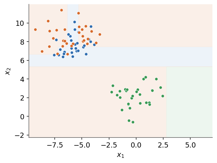	*Un arbre découpe l'espace en régions alignées sur les axes, chacune à prédiction constante.*
-	## 5.2 Forêts aléatoires
+	## 7.2 Forêts aléatoires
-	### 5.2.1 Bagging
+	### 7.2.1 Bagging
	Le bagging (bootstrap aggregating) entraîne $B$ arbres sur $B$ rééchantillons bootstrap des données et les moyenne. Le prédicteur agrégé est défini par
@@ 84,7 84,7 @@
	Un échantillon bootstrap tire $N$ exemples avec remise parmi $N$ exemples. La probabilité qu'un exemple donné ne soit jamais tiré vaut $(1-\tfrac1N)^N\to e^{-1}\approx0{,}37$, donc environ 37 % des données restent hors de chaque arbre. Ce sont ses exemples hors-sac (OOB).
-	### 5.2.2 Variance d'une moyenne
+	### 7.2.2 Variance d'une moyenne
	Si les $B$ arbres ont chacun une variance $\sigma^2$ et une corrélation deux à deux $\rho$, la variance de leur moyenne vaut
@@ 92,7 92,7 @@
	Le second terme s'annule quand $B$ croît, mais le premier, $\rho\sigma^2$, persiste. Réduire la corrélation $\rho$ entre les arbres est donc le levier clé, et c'est précisément ce que visent les forêts aléatoires.
-	### 5.2.3 Forêts aléatoires
+	### 7.2.3 Forêts aléatoires
	Une forêt aléatoire est du bagging avec sous-échantillonnage des variables : à chaque coupure, seul un sous-ensemble aléatoire de $m_{\text{try}}$ variables est considéré comme candidat. Les choix usuels sont
@@ 122,13 122,13 @@
	T3 --> AGG
	```
-	
+	
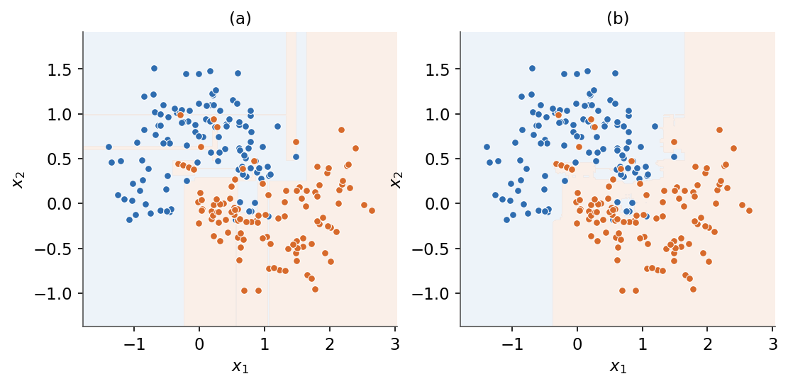	*(a) Un arbre profond seul surajuste avec une frontière en escalier. (b) Une forêt aléatoire moyenne de nombreux arbres pour une frontière plus lisse.*
-	## 5.3 Boosting
+	## 7.3 Boosting
-	### 5.3.1 Modèle additif
+	### 7.3.1 Modèle additif
	Le boosting construit un prédicteur comme une somme pondérée de $T$ apprenants faibles $h_t$ (typiquement des arbres peu profonds), ajustés un à un. Le modèle additif est défini par
@@ 136,7 136,7 @@
	Chaque étape corrige les erreurs de la somme courante, donc l'ensemble est construit de façon séquentielle et réduit le biais plutôt que la variance.
-	### 5.3.2 AdaBoost
+	### 7.3.2 AdaBoost
	Avec des étiquettes $y\in\{-1,+1\}$, AdaBoost conserve des poids d'exemples $w^{(i)}$ qui se concentrent sur les points actuellement mal classés. Au tour $t$, l'apprenant faible a une erreur pondérée $\varepsilon_t$, et son coefficient est défini par
@@ 148,7 148,7 @@
	puis renormalisés. Les exemples mal classés ($y^{(i)}h_t(x^{(i)})<0$) gagnent du poids, donc l'apprenant suivant se concentre sur eux.
-	### 5.3.3 Gradient boosting
+	### 7.3.3 Gradient boosting
	Le gradient boosting généralise l'idée à toute perte différentiable $L$. À l'étape $t$, il ajuste l'apprenant suivant sur l'opposé du gradient de la perte évalué au modèle courant, le pseudo-résidu défini par
fr/Machine Learning/05 Decision trees and ensemble methods/forest-vs-tree.png .. fr/Machine Learning/07 Decision trees and ensemble methods/forest-vs-tree.png
fr/Machine Learning/05 Decision trees and ensemble methods/tree-boundary.png .. fr/Machine Learning/07 Decision trees and ensemble methods/tree-boundary.png