Commit 6b31d5
2026-07-15 12:37:13 lugonthier: feat: Update "Decision trees and ensemble methods" module with new content and visuals - Revamped the introduction to ensemble methods, emphasizing the benefits of combining models. - Expanded sections on decision trees, bagging, and boosting, including detailed explanations and formulas. - Added new SVG diagrams illustrating the bagging process, the transition from stumps to trees, and variance reduction. - Introduced new images for AdaBoost rounds and variance reduction to enhance understanding.| en/Deep Learning.md .. | |
| @@ 16,12 16,11 @@ | |
| 8. [Normalization](/en/Deep%20Learning/08%20Normalization) | |
| 9. [Regularization and dropout](/en/Deep%20Learning/09%20Regularization%20and%20dropout) | |
| 10. [Convolutional networks](/en/Deep%20Learning/10%20Convolutional%20networks) | |
| - | 11. [CNN architectures](/en/Deep%20Learning/11%20CNN%20architectures) |
| - | 12. [Embeddings and representation learning](/en/Deep%20Learning/12%20Embeddings%20and%20representation%20learning) |
| - | 13. [Recurrent networks](/en/Deep%20Learning/13%20Recurrent%20networks) |
| - | 14. [LSTM and GRU](/en/Deep%20Learning/14%20LSTM%20and%20GRU) |
| - | 15. [Attention](/en/Deep%20Learning/15%20Attention) |
| - | 16. [Transformers](/en/Deep%20Learning/16%20Transformers) |
| + | 11. [Embeddings and representation learning](/en/Deep%20Learning/11%20Embeddings%20and%20representation%20learning) |
| + | 12. [Recurrent networks](/en/Deep%20Learning/12%20Recurrent%20networks) |
| + | 13. [LSTM and GRU](/en/Deep%20Learning/13%20LSTM%20and%20GRU) |
| + | 14. [Attention](/en/Deep%20Learning/14%20Attention) |
| + | 15. [Transformers](/en/Deep%20Learning/15%20Transformers) |
| --- | |
| [Machine Learning](/en/Machine%20Learning) · [MLOps](/en/MLOps) · [Home](/en) | |
| en/Deep Learning/01 Introduction.md .. | |
| @@ 11,13 11,13 @@ | |
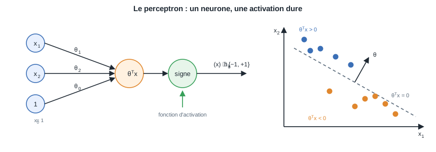
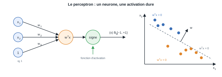
| ## 1.1 The perceptron, recalled | |
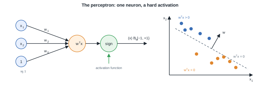
| - | The perceptron from the Machine Learning course is a single computational unit. It scores an input with a linear combination of its features and passes that score through a hard threshold. With parameters $\theta$ and the step activation $g$, its hypothesis is: |
| + | The perceptron from the Machine Learning course is a single computational unit. It scores an input with a linear combination of its features and passes that score through a hard threshold. With parameters $w$ and the step activation $g$, its hypothesis is: |
| - | $$\boxed{ h(x) = g(\theta^T x), \quad g(z) = \begin{cases} 1 & \text{if } z \ge 0 \\ 0 & \text{otherwise} \end{cases} }$$ |
| + | $$\boxed{ h(x) = g(w^T x), \quad g(z) = \begin{cases} 1 & \text{if } z \ge 0 \\ 0 & \text{otherwise} \end{cases} }$$ |
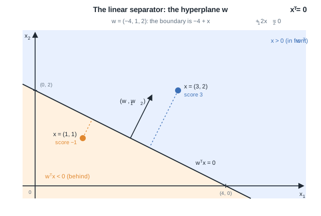
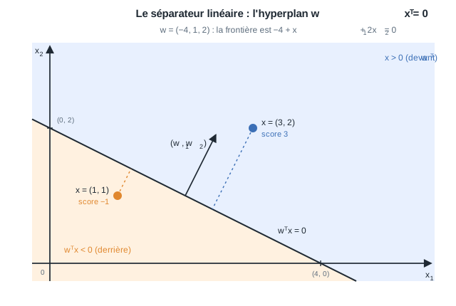
| - | The equation $\theta^T x = 0$ is a hyperplane, so the perceptron splits the input space with a single flat boundary. Points on one side are labelled $1$, points on the other are labelled $0$. |
| + | The equation $w^T x = 0$ is a hyperplane, so the perceptron splits the input space with a single flat boundary. Points on one side are labelled $1$, points on the other are labelled $0$. |
| - | *Remark:* the boundary is linear because the score $\theta^T x$ is linear in $x$. The threshold only chooses a side, it does not bend the boundary. |
| + | *Remark:* the boundary is linear because the score $w^T x$ is linear in $x$. The threshold only chooses a side, it does not bend the boundary. |
| ## 1.2 Why one unit is not enough | |
| @@ 52,7 52,7 @@ | |
| ## 1.4 Notation for this course | |
| - | The Machine Learning course folded the bias into the score with the intercept convention $x_0 = 1$, so a single dot product $\theta^T x$ carried the constant term. This course keeps the bias **explicit** and uses a separate weight matrix per layer. This is the seam between the two courses: from here on, no augmented input and no folded bias. |
| + | The Machine Learning course folded the bias into the score with the intercept convention $x_0 = 1$, so a single dot product $w^T x$ carried the constant term. This course keeps the bias **explicit** and uses a separate weight matrix per layer. This is the seam between the two courses: from here on, no augmented input and no folded bias. |
| ### 1.4.1 A single unit | |
| @@ 60,7 60,7 @@ | |
| $$\boxed{ a = g(w^T x + b) }$$ | |
| - | The score $w^T x + b$ is the same affine function as before, only now the bias $b$ is written out instead of hidden inside $\theta$. |
| + | The score $w^T x + b$ is the same affine function as before, only now the bias $b$ is written out instead of hidden inside $w$. |
| ### 1.4.2 A layer and a network | |
| en/Deep Learning/02 Multilayer perceptron.md .. | |
| @@ 27,7 27,7 @@ | |
| The whole layer then computes a pre-activation vector and an activation vector in one matrix expression, $z^{[1]} = W^{[1]} x + b^{[1]}$ and $a^{[1]} = g^{[1]}(z^{[1]})$, where $g^{[1]}$ is applied elementwise. | |
| - | *Remark:* the rows of $W^{[1]}$ are exactly the individual unit weight vectors, so a layer is just many units packed into one matrix. Bias stays explicit here: unlike the Machine Learning course, which folded the intercept into $\theta$ via the augmented input $x_0 = 1$, this course keeps $b^{[l]}$ as its own vector. |
| + | *Remark:* the rows of $W^{[1]}$ are exactly the individual unit weight vectors, so a layer is just many units packed into one matrix. Bias stays explicit here: unlike the Machine Learning course, which folded the intercept into $w$ via the augmented input $x_0 = 1$, this course keeps $b^{[l]}$ as its own vector. |
| ## 2.2 Forward propagation | |
| en/Deep Learning/03 Activation functions.md .. | |
| @@ 17,7 17,7 @@ | |
| with $W' = W^{[L]} \cdots W^{[1]}$ and $b'$ the accumulated bias. No matter how many linear layers are stacked, the model can only fit a linear function, so the extra depth buys nothing. A nonlinear $g$ between layers is exactly what breaks this collapse and lets the network represent curved decision boundaries and nonlinear regressions. | |
| - | *Remark:* the bias is kept explicit here as $b^{[l]}$, unlike the Machine Learning course where the intercept was folded into $\theta^T x$ via the augmented input $x_0 = 1$. In this Deep Learning course each layer has its own weight matrix $W^{[l]}$ and its own bias vector $b^{[l]}$. |
| + | *Remark:* the bias is kept explicit here as $b^{[l]}$, unlike the Machine Learning course where the intercept was folded into $w^T x$ via the augmented input $x_0 = 1$. In this Deep Learning course each layer has its own weight matrix $W^{[l]}$ and its own bias vector $b^{[l]}$. |
| ## 3.2 Sigmoid and tanh | |
| en/Deep Learning/06 Optimization.md .. | |
| @@ 12,9 12,9 @@ | |
| ## 6.1 Gradient descent | |
| - | Let $\theta$ collect all parameters (every $W^{[l]}$ and $b^{[l]}$) and let $J(\theta)$ be the cost, the average of the per-example loss $L$. Write $g = \nabla_\theta J(\theta)$ for the gradient of the cost with respect to the parameters, as returned by backpropagation. The base update moves $\theta$ downhill: |
| + | Let $w$ collect all parameters (every $W^{[l]}$ and $b^{[l]}$) and let $J(w)$ be the cost, the average of the per-example loss $L$. Write $g = \nabla_w J(w)$ for the gradient of the cost with respect to the parameters, as returned by backpropagation. The base update moves $w$ downhill: |
| - | $$\boxed{ \theta \leftarrow \theta - \alpha\, g }$$ |
| + | $$\boxed{ w \leftarrow w - \alpha\, g }$$ |
| with learning rate $\alpha > 0$. This is the LMS update from the Machine Learning course, written for the full parameter vector instead of one coordinate. | |
| @@ 36,15 36,15 @@ | |
| Plain SGD zig-zags across narrow valleys because the gradient points across the valley more than along it. Momentum accumulates an exponentially weighted average of past gradients in a velocity vector $v$, then steps in that averaged direction: | |
| - | $$\boxed{ v \leftarrow \beta\, v + g, \qquad \theta \leftarrow \theta - \alpha\, v }$$ |
| + | $$\boxed{ v \leftarrow \beta\, v + g, \qquad w \leftarrow w - \alpha\, v }$$ |
| with momentum coefficient $\beta \in [0, 1)$, typically $\beta = 0.9$. Components of $g$ that keep the same sign reinforce each other, so $v$ grows and the step accelerates along consistent directions. Components that flip sign cancel in the average, so oscillations across the valley are damped. | |
| ### 6.2.1 Nesterov momentum | |
| - | Nesterov accelerated gradient evaluates the gradient at a look-ahead point, after the momentum step has been provisionally applied, rather than at the current $\theta$. This anticipatory correction reacts sooner when the slope changes: |
| + | Nesterov accelerated gradient evaluates the gradient at a look-ahead point, after the momentum step has been provisionally applied, rather than at the current $w$. This anticipatory correction reacts sooner when the slope changes: |
| - | $$\boxed{ v \leftarrow \beta\, v + \nabla_\theta J(\theta - \alpha \beta\, v), \qquad \theta \leftarrow \theta - \alpha\, v }$$ |
| + | $$\boxed{ v \leftarrow \beta\, v + \nabla_w J(w - \alpha \beta\, v), \qquad w \leftarrow w - \alpha\, v }$$ |
| *Remark:* think of $\beta \approx 0.9$ as averaging over roughly the last $\tfrac{1}{1 - \beta} = 10$ gradients. Nesterov usually converges slightly faster than plain momentum for the same $\alpha$ and $\beta$. | |
| @@ 52,7 52,7 @@ | |
| Different parameters can need very different step sizes, and one global $\alpha$ cannot serve them all. RMSProp keeps a per-coordinate running average $s$ of squared gradients, then divides the step by $\sqrt{s}$, so coordinates with large recent gradients take smaller steps and quiet coordinates take larger ones: | |
| - | $$\boxed{ s \leftarrow \rho\, s + (1 - \rho)\, g^2, \qquad \theta \leftarrow \theta - \alpha\, \frac{g}{\sqrt{s} + \epsilon} }$$ |
| + | $$\boxed{ s \leftarrow \rho\, s + (1 - \rho)\, g^2, \qquad w \leftarrow w - \alpha\, \frac{g}{\sqrt{s} + \epsilon} }$$ |
| with decay $\rho \approx 0.9$ and a small $\epsilon \approx 10^{-8}$ for numerical safety. Here $g^2 = g \odot g$ is the Hadamard (elementwise) square and the division is elementwise, so each coordinate is normalized by its own recent gradient scale. | |
| @@ 70,7 70,7 @@ | |
| The update then steps in the momentum direction, rescaled per coordinate by the second moment: | |
| - | $$\boxed{ \theta \leftarrow \theta - \alpha\, \frac{\hat m}{\sqrt{\hat v} + \epsilon} }$$ |
| + | $$\boxed{ w \leftarrow w - \alpha\, \frac{\hat m}{\sqrt{\hat v} + \epsilon} }$$ |
| Common defaults are $\beta_1 = 0.9$, $\beta_2 = 0.999$, and $\epsilon = 10^{-8}$. As before the square, square root, and division are elementwise. | |
| en/Deep Learning/10 Convolutional networks.md .. | |
| @@ 9,6 9,7 @@ | |
| - Extend a filter to multiple input and output channels (feature maps). | |
| - Use max and average pooling to downsample and add small translation invariance. | |
| - Compare the parameter count of a convolution against an equivalent dense layer. | |
| + | - Recognize the landmark architectures, LeNet to ResNet, and the one idea each contributed. |
| ## 10.1 Why not a dense layer | |
| @@ 106,7 107,41 @@ | |
| *Remark:* stacking such stages makes the receptive field (the input region that influences one output value) grow with depth, so early layers see edges and deep layers see whole objects, all built from the same local operation. | |
| - | *One convolution and pooling stage is the building block. The next part assembles many of them into the classic designs, from LeNet and AlexNet to residual networks.* |
| + | ## 10.8 From layers to architectures |
| + | |
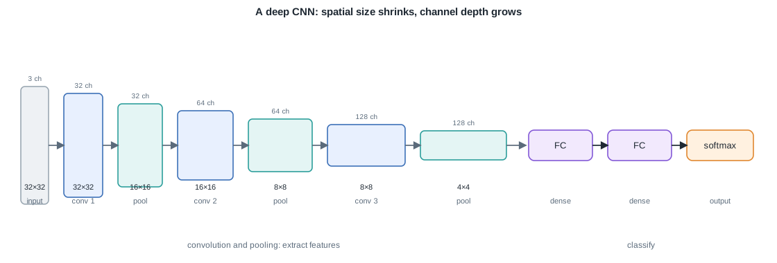
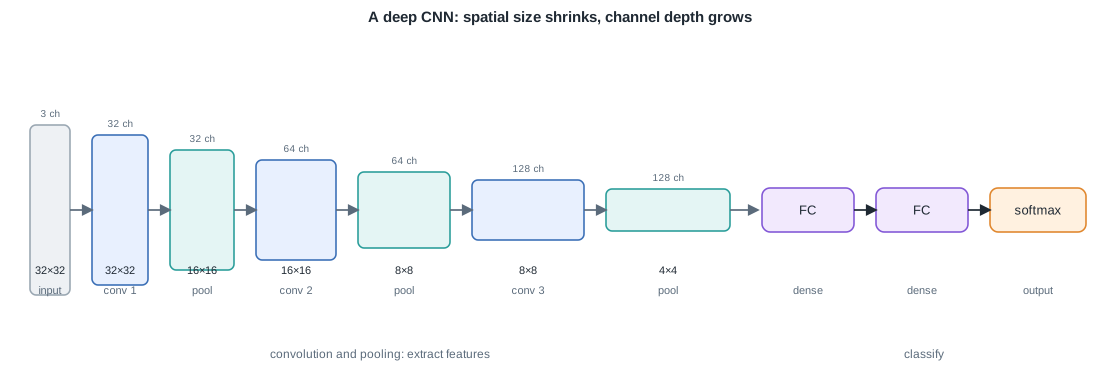
| + | The landmark convolutional networks all share one shape: a stack of convolution and pooling stages that extracts features, then a small fully connected head that classifies them. |
| + | |
| + |  |
| + | |
| + | *A deep CNN progressively reduces spatial size while increasing channel depth, then flattens into fully connected layers.* |
| + | |
| + | Each generation contributed one idea to the same question, how to stack more layers without the training signal decaying: |
| + | |
| + | - **LeNet**, the original, alternates a handful of convolution and pooling stages for digit recognition. |
| + | - **AlexNet** scaled that skeleton to large images and GPUs, made trainable by ReLU activations and dropout. |
| + | - **VGG** made every convolution $3 \times 3$ and got its depth by stacking: two $3 \times 3$ layers see the same region as one $5 \times 5$ with fewer parameters ($18c^2$ against $25c^2$) and one more nonlinearity. |
| + | - **Inception** runs branches of several filter sizes in parallel and concatenates them, kept affordable by $1 \times 1$ convolutions, per-position channel maps that squeeze a thick feature map down before the expensive filters. |
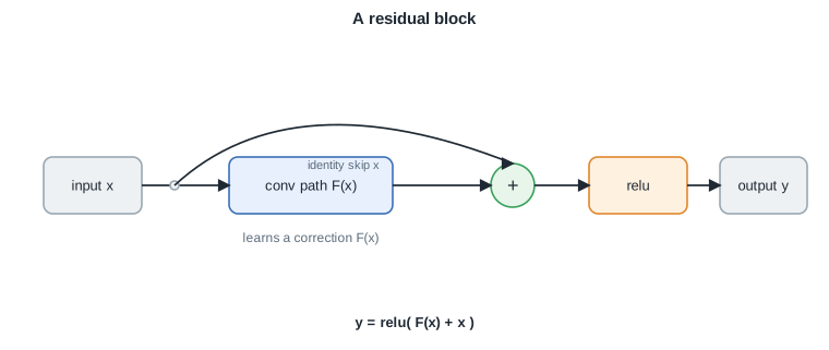
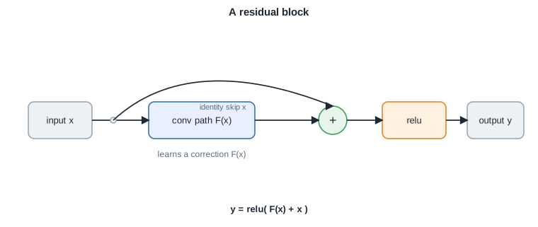
| + | - **ResNet** lets each block learn a correction around an identity skip connection: |
| + | |
| + | $$\boxed{\ y = F(x, W) + x, \qquad \frac{\partial y}{\partial x} = \frac{\partial F}{\partial x} + I\ }$$ |
| + | |
| + | The $+I$ gives the gradient a backward route that never shrinks, the direct remedy to the [vanishing gradient](/en/Deep%20Learning/07%20Initialization%20and%20vanishing%20gradients) of lesson 7, and networks of hundreds of layers train reliably. |
| + | |
| + |  |
| + | |
| + | *A residual block adds an identity skip connection around the convolution path, so the layer only has to learn a correction F(x).* |
| + | |
| + | | Architecture | Approx. depth | Key idea | |
| + | | --- | --- | --- | |
| + | | LeNet | 5 to 7 layers | conv and pool stack | |
| + | | AlexNet | 8 layers | ReLU and dropout at scale | |
| + | | VGG | 16 to 19 layers | stacks of $3 \times 3$ convolutions | |
| + | | Inception | 22 layers | parallel branches, $1 \times 1$ bottleneck | |
| + | | ResNet | 50 to 152 layers | residual skip connections | |
| + | |
| + | *Remark:* the trend is monotonic in depth, and each jump was unlocked by a specific fix: better activations, smaller filters, channel bottlenecks, and finally skip connections. |
| + | |
| + | *These deep stacks learn feature maps whose deeper activations behave as reusable representations, the entry point of the next module on embeddings and representation learning.* |
| --- | |
| - | Next: [CNN architectures](/en/Deep%20Learning/11%20CNN%20architectures) · [Course overview](/en/Deep%20Learning) |
| + | Next: [Embeddings and representation learning](/en/Deep%20Learning/11%20Embeddings%20and%20representation%20learning) · [Course overview](/en/Deep%20Learning) |
| en/Deep Learning/11 CNN architectures/cnn-stack.svg .. en/Deep Learning/10 Convolutional networks/cnn-stack.svg | |
| en/Deep Learning/11 CNN architectures/residual-block.svg .. en/Deep Learning/10 Convolutional networks/residual-block.svg | |
| en/Deep Learning/11 CNN architectures.md .. /dev/null | |
| @@ 1,99 0,0 @@ | |
| - | # 11. CNN architectures |
| - | |
| - | The layers and operations of the previous module compose into full networks, and a handful of landmark architectures shaped how those pieces are assembled. This module surveys LeNet, AlexNet, VGG, Inception, and ResNet, extracting the one idea each contributed. The through-line is a search for depth: how to stack more layers without the training signal decaying, which ties directly back to the vanishing-gradient problem of lesson 7. |
| - | |
| - | **Objectives** |
| - | - Trace the progression from the early convolutional stacks of LeNet and AlexNet. |
| - | - Explain why VGG replaced large filters with deep stacks of small $3 \times 3$ convolutions. |
| - | - Read an Inception module as parallel branches and understand the $1 \times 1$ convolution as a channel bottleneck. |
| - | - Write the residual block $y = F(x, W) + x$ and connect the skip connection to gradient flow. |
| - | - Compare the five architectures by depth, key idea, and contribution. |
| - | |
| - | All of these architectures share the same overall shape: a stack of convolution and pooling layers that extract features, followed by a small fully connected head that classifies them. |
| - | |
| - |  |
| - | |
| - | *A deep CNN progressively reduces spatial size while increasing channel depth, then flattens into fully connected layers.* |
| - | |
| - | ## 11.1 Early convolutional stacks |
| - | |
| - | ### 11.1.1 LeNet |
| - | |
| - | LeNet is the original convolutional network, built for handwritten-digit recognition. It alternates convolution and pooling layers to extract features, then finishes with fully connected layers for classification. A layer $l$ still computes $z^{[l]} = W^{[l]} a^{[l-1]} + b^{[l]}$ followed by $a^{[l]} = g^{[l]}(z^{[l]})$, but $W^{[l]}$ is now a bank of small shared filters rather than a dense matrix. The activation $g^{[l]}$ was a saturating sigmoid or $\tanh$, and the whole network was only a handful of layers deep. |
| - | |
| - | ### 11.1.2 AlexNet |
| - | |
| - | AlexNet kept the convolution-then-pool skeleton but scaled it to large natural images and trained it on GPUs. Two ideas from this course made deep training practical at that scale. First, the ReLU activation |
| - | |
| - | $$\boxed{\ g(z) = \max(0, z)\ }$$ |
| - | |
| - | replaced the saturating sigmoid, so the gradient is $1$ wherever $z > 0$ and does not vanish for large positive inputs. Second, dropout randomly zeroes a fraction $p$ of activations during training, which regularizes the large fully connected layers: |
| - | |
| - | $$\boxed{\ a^{[l]} \leftarrow \frac{1}{1-p}\, m \odot a^{[l]}, \quad m_j \sim \text{Bernoulli}(1-p)\ }$$ |
| - | |
| - | *Remark:* the mask $m$ is applied elementwise with the Hadamard product $\odot$, and the $1/(1-p)$ factor keeps the expected activation unchanged so that no rescaling is needed at test time. |
| - | |
| - | ## 11.2 VGG: depth from small filters |
| - | |
| - | VGG made one design choice and pushed it hard: every convolution is $3 \times 3$, and depth comes from stacking many of them. Two stacked $3 \times 3$ convolutions see the same input region as one $5 \times 5$ convolution, and three stacked see the same region as one $7 \times 7$. The stack is cheaper and more expressive, because it inserts a nonlinearity between each layer while using fewer parameters. |
| - | |
| - | For a filter of side $k$ mapping $c_{\text{in}}$ input channels to $c_{\text{out}}$ output channels, the weight count is |
| - | |
| - | $$\boxed{\ \#\text{params} = k^2 \cdot c_{\text{in}} \cdot c_{\text{out}} \ }$$ |
| - | |
| - | so with $c_{\text{in}} = c_{\text{out}} = c$ a single $5 \times 5$ layer costs $25 c^2$ weights, while two $3 \times 3$ layers cost $2 \cdot 9 c^2 = 18 c^2$. The deeper stack is both smaller and adds an extra ReLU. |
| - | |
| - | *Remark:* the regular structure is what made VGG a favourite backbone. The trade is cost, because its wide fully connected head holds most of the parameters. |
| - | |
| - | ## 11.3 Inception: parallel branches and the 1x1 convolution |
| - | |
| - | Instead of choosing a single filter size, an Inception module (GoogLeNet) runs several in parallel and concatenates their outputs along the channel axis. One branch is $1 \times 1$, one is $3 \times 3$, one is $5 \times 5$, and one is a pooling branch, so the network learns which scale matters at each stage rather than fixing it by hand. |
| - | |
| - | The key trick is the $1 \times 1$ convolution. It has no spatial extent, so it does not mix neighbouring pixels. Instead it acts as a per-position linear map across channels, computing at each spatial location $(i, j)$ |
| - | |
| - | $$\boxed{\ y_{ij} = W\, a_{ij} + b, \quad W \in \mathbb{R}^{c_{\text{out}} \times c_{\text{in}}}\ }$$ |
| - | |
| - | Choosing $c_{\text{out}} < c_{\text{in}}$ makes it a channel bottleneck: it projects a thick feature map down to fewer channels before an expensive $3 \times 3$ or $5 \times 5$ convolution, cutting the cost of that convolution sharply. This is why Inception can be both wide and affordable. |
| - | |
| - | *Remark:* a $1 \times 1$ convolution followed by a ReLU is exactly a small fully connected network applied identically at every spatial position, sharing one weight matrix $W$ across the whole feature map. |
| - | |
| - | ## 11.4 ResNet: residual connections |
| - | |
| - | ### 11.4.1 The residual block |
| - | |
| - | Very deep plain stacks train worse than shallow ones, not because they overfit but because the signal degrades. ResNet fixes this by having each block learn a residual and adding the input back through a skip connection: |
| - | |
| - | $$\boxed{\ y = F(x, W) + x\ }$$ |
| - | |
| - | Here $F$ is a short stack of convolutions with weights $W$, and the term $+x$ is the identity skip. If the optimal map for a block is close to the identity, the network only has to drive $F$ toward zero, which is far easier than learning the identity from scratch through several nonlinear layers. |
| - | |
| - |  |
| - | |
| - | *A residual block adds an identity skip connection around the convolution path, so the layer only has to learn a correction F(x).* |
| - | |
| - | ### 11.4.2 Why gradients flow |
| - | |
| - | Differentiating the block, the skip contributes an identity term to the Jacobian: |
| - | |
| - | $$\boxed{\ \frac{\partial y}{\partial x} = \frac{\partial F}{\partial x} + I\ }$$ |
| - | |
| - | During backpropagation the upstream gradient is multiplied by this factor at every block. The $+I$ term gives the gradient a direct route backward that never shrinks, so even when the $\partial F / \partial x$ contributions are small the product across many blocks does not collapse toward zero. This is the direct remedy to the vanishing-gradient problem from lesson 7, where repeated multiplication by small Jacobians in a plain deep stack drives early-layer gradients to nothing. With skip connections, networks of hundreds of layers train reliably. |
| - | |
| - | *Remark:* when $F$ changes the number of channels or the spatial size, the skip uses a $1 \times 1$ convolution to match shapes so the sum $F(x, W) + x$ is well defined. |
| - | |
| - | ## 11.5 Comparison |
| - | |
| - | | Architecture | Approx. depth | Key idea | Contribution | |
| - | | --- | --- | --- | --- | |
| - | | LeNet | 5 to 7 layers | conv and pool stack | first working CNN for digits | |
| - | | AlexNet | 8 layers | ReLU and dropout at scale | deep CNNs on large images and GPUs | |
| - | | VGG | 16 to 19 layers | stacks of $3 \times 3$ convolutions | depth from uniform small filters | |
| - | | Inception | 22 layers | multi-branch modules, $1 \times 1$ bottleneck | width and efficiency together | |
| - | | ResNet | 50 to 152 layers | residual block $y = F(x, W) + x$ | trains very deep networks | |
| - | |
| - | *Remark:* the trend is monotonic in depth, and each jump was unlocked by a specific fix, better activations, smaller filters, channel bottlenecks, and finally skip connections. |
| - | |
| - | *These architectures learn hierarchical feature maps whose deeper activations behave as reusable representations, which is the entry point to the next module on embeddings and representation learning.* |
| - | |
| - | --- |
| - | Next: [Embeddings and representation learning](/en/Deep%20Learning/12%20Embeddings%20and%20representation%20learning) · [Course overview](/en/Deep%20Learning) |
| en/Deep Learning/12 Embeddings and representation learning.md .. en/Deep Learning/11 Embeddings and representation learning.md | |
| @@ 1,4 1,4 @@ | |
| - | # 12. Embeddings and representation learning |
| + | # 11. Embeddings and representation learning |
| Neural networks turn raw inputs into useful features by learning them rather than hand-crafting them. For discrete symbols (words, product IDs, user IDs, categories) the natural representation is a learned dense vector called an embedding. This lesson shows why one-hot codes are a poor input, how an embedding matrix maps each symbol to a compact vector, how word2vec learns such vectors from co-occurrence, and why embeddings are the standard input to the sequence models and Transformers that follow. | |
| @@ 10,9 10,9 @@ | |
| - See how the same idea covers items, users, and categorical features. | |
| - Connect embeddings to recurrent networks and Transformers as the input layer. | |
| - | ## 12.1 From one-hot to dense vectors |
| + | ## 11.1 From one-hot to dense vectors |
| - | ### 12.1.1 The one-hot representation |
| + | ### 11.1.1 The one-hot representation |
| Suppose the vocabulary has $V$ distinct symbols. The classic way to feed symbol $i$ to a network is the one-hot vector $x_{\text{onehot}} \in \{0, 1\}^V$, which is all zeros except for a single $1$ at position $i$. It carries no structure: every pair of distinct symbols is exactly as far apart as every other pair, so the code holds no notion of similarity. It is also enormous, a modern vocabulary has $V$ in the tens or hundreds of thousands, and it is almost entirely zeros. | |
| @@ 26,7 26,7 @@ | |
| *Remark:* feeding a one-hot vector into a linear layer $W x_{\text{onehot}}$ simply selects one column of $W$. The embedding lookup below makes that selection explicit and cheap. | |
| - | ### 12.1.2 The embedding lookup |
| + | ### 11.1.2 The embedding lookup |
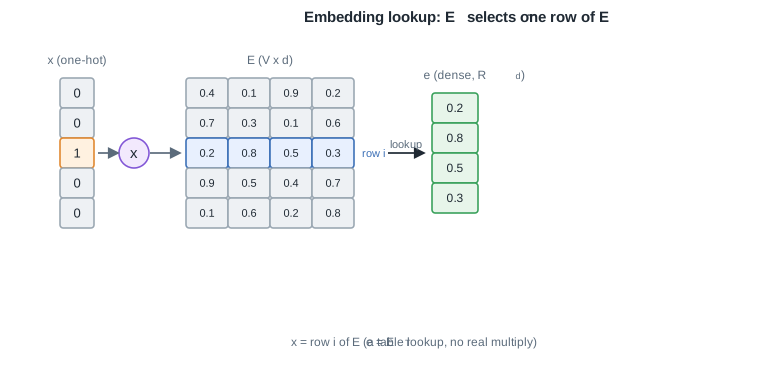
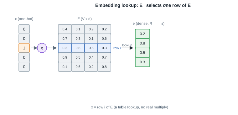
| An embedding matrix $E \in \mathbb{R}^{V \times d}$ stores one $d$-dimensional row per symbol. The embedding of a one-hot input is the matrix-vector product | |
| @@ 36,11 36,11 @@ | |
| *Remark:* the rows of $E$ are ordinary parameters. They start random and are updated by backpropagation together with the rest of the network, so the geometry of the space is shaped by whatever task the network is trained on. | |
| - | ## 12.2 Learning word embeddings with word2vec |
| + | ## 11.2 Learning word embeddings with word2vec |
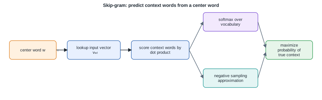
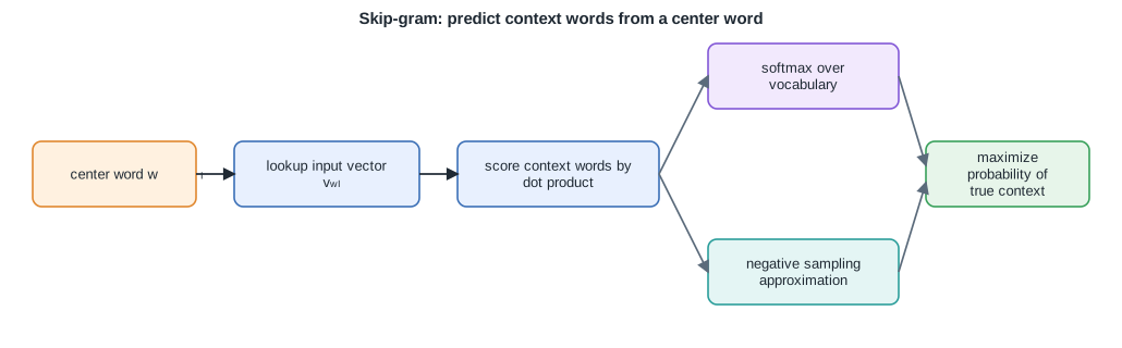
| Embeddings can be learned end to end inside any task, but they can also be learned on their own from unlabelled text. The word2vec skip-gram model does exactly this: it learns a vector per word by predicting the surrounding context words from a centre word. | |
| - | ### 12.2.1 Skip-gram objective |
| + | ### 11.2.1 Skip-gram objective |
| Each word $w$ has an input vector $v_w$ (its row in the embedding matrix). Given a centre word $w_I$, the model scores each candidate output word $w_O$ by a dot product and normalizes over the whole vocabulary with a softmax: | |
| @@ 48,17 48,17 @@ | |
| Training maximizes this probability for the (centre, context) pairs that actually co-occur in a sliding window over the text. Words that appear in similar contexts are pushed to have large dot products, so their vectors end up close together. | |
| - | ### 12.2.2 Negative sampling |
| + | ### 11.2.2 Negative sampling |
| The denominator sums over all $V$ words, which is far too expensive to compute for every training pair. Negative sampling replaces the full softmax with a cheap binary problem: for each real (centre, context) pair, draw a few random words as negatives and train the model to tell the true context word from the fakes. This turns one $V$-way normalization into a handful of logistic updates per step and is what makes word2vec fast enough to train on billions of words. | |
| - |  |
| + |  |
| *The skip-gram model learns embeddings by predicting a word context from a center word.* | |
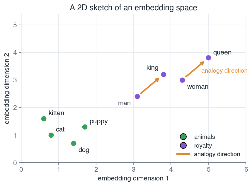
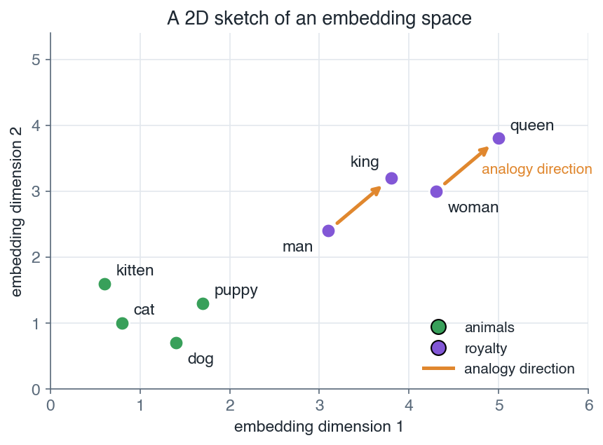
| *Remark:* the learned space has a striking linear structure. Directions in it encode consistent relations, so analogies show up as vector arithmetic, the classic example being that the vector for "king" minus "man" plus "woman" lands near "queen". | |
| - | ## 12.3 Measuring similarity |
| + | ## 11.3 Measuring similarity |
| Once symbols are dense vectors, "how related are two symbols" becomes a geometric question. The standard answer is cosine similarity, the cosine of the angle between two vectors $u$ and $v$: | |
| @@ 66,13 66,13 @@ | |
| It lies in $[-1, 1]$: a value near $1$ means the vectors point the same way (very similar), near $0$ means unrelated, and near $-1$ means opposite. Cosine ignores vector length and looks only at direction, which is usually what we want, since a word's meaning should not depend on how often it appears. | |
| - |  |
| + |  |
| *Learned embeddings place related words near each other, and consistent directions in the space capture analogies.* | |
| *Remark:* nearest-neighbour search under cosine similarity is how embeddings power retrieval and recommendation. Find the stored vectors whose direction is closest to a query vector and you have the most relevant items. | |
| - | ## 12.4 Embeddings beyond words |
| + | ## 11.4 Embeddings beyond words |
| Nothing in the construction is specific to language. Any set of discrete symbols can be embedded by giving it a matrix $E$ and learning its rows. | |
| @@ 91,11 91,11 @@ | |
| *Remark:* embeddings are also a form of dimensionality reduction. They compress a $V$-way symbol into $d$ numbers while keeping the information a downstream task needs, which is the essence of representation learning. | |
| - | ## 12.5 Embeddings as the input to sequence models |
| + | ## 11.5 Embeddings as the input to sequence models |
| - | A sequence of symbols becomes a sequence of vectors by looking each one up in $E$. That matrix of embeddings is exactly the input a recurrent network reads step by step (lesson [Recurrent networks](/en/Deep%20Learning/13%20Recurrent%20networks)) and the input a Transformer attends over (lesson [Transformers](/en/Deep%20Learning/16%20Transformers)). In both cases the embedding table is learned jointly with the rest of the model, so the representations are tuned to the end task rather than fixed in advance. |
| + | A sequence of symbols becomes a sequence of vectors by looking each one up in $E$. That matrix of embeddings is exactly the input a recurrent network reads step by step (lesson [Recurrent networks](/en/Deep%20Learning/12%20Recurrent%20networks)) and the input a Transformer attends over (lesson [Transformers](/en/Deep%20Learning/15%20Transformers)). In both cases the embedding table is learned jointly with the rest of the model, so the representations are tuned to the end task rather than fixed in advance. |
| - |  |
| + |  |
| *An embedding lookup selects one row of the matrix E, mapping a sparse one-hot token to a dense learned vector.* | |
| @@ 104,4 104,4 @@ | |
| *Dense vectors give us a compact, similarity-aware input. The next lesson feeds such a sequence of vectors, one step at a time, into a recurrent network that carries a hidden state through time.* | |
| --- | |
| - | Next: [Recurrent networks](/en/Deep%20Learning/13%20Recurrent%20networks) · [Course overview](/en/Deep%20Learning) |
| \ | No newline at end of file |
| + | Next: [Recurrent networks](/en/Deep%20Learning/12%20Recurrent%20networks) · [Course overview](/en/Deep%20Learning) |
| \ | No newline at end of file |
| en/Deep Learning/12 Embeddings and representation learning/embedding-lookup.svg .. en/Deep Learning/11 Embeddings and representation learning/embedding-lookup.svg | |
| en/Deep Learning/12 Embeddings and representation learning/embedding-space.png .. en/Deep Learning/11 Embeddings and representation learning/embedding-space.png | |
| en/Deep Learning/12 Embeddings and representation learning/skipgram.svg .. en/Deep Learning/11 Embeddings and representation learning/skipgram.svg | |
| en/Deep Learning/13 Recurrent networks.md .. en/Deep Learning/12 Recurrent networks.md | |
| @@ 1,4 1,4 @@ | |
| - | # 13. Recurrent networks |
| + | # 12. Recurrent networks |
| Feedforward and convolutional networks map a fixed-size input to an output in one pass, but many problems come as sequences whose length varies and whose order matters (text, audio, time series). A recurrent neural network (RNN) processes a sequence one step at a time and carries a hidden state forward, so past inputs influence the current output. This module introduces recurrence, the vanilla RNN cell, how it is trained by backpropagation through time, and why long-range gradients tend to vanish or explode. | |
| @@ 9,7 9,7 @@ | |
| - Derive how backpropagation through time (BPTT) accumulates the gradient over all steps. | |
| - Diagnose vanishing and exploding gradients from the product of Jacobians over time. | |
| - | ## 13.1 Sequence data and memory |
| + | ## 12.1 Sequence data and memory |
| A sequence is an ordered list of inputs $x_1, x_2, \dots, x_T$, where $T$ can differ from one example to the next. A feedforward network of the kind seen in earlier lessons expects a single fixed-size vector $a^{[0]} = x$, so it has no natural way to consume a variable-length input or to remember what came before the current element. | |
| @@ 24,9 24,9 @@ | |
| | Many to many (seq2seq) | sequence | sequence, other length | machine translation | | |
| | One to many | single vector | sequence | image captioning | | |
| - | ## 13.2 The vanilla RNN cell |
| + | ## 12.2 The vanilla RNN cell |
| - | ### 13.2.1 Recurrence |
| + | ### 12.2.1 Recurrence |
| At step $t$ the cell reads the current input $x_t$ and the previous hidden state $h_{t-1}$, then produces a new hidden state through an activation $g$ (usually $\tanh$): | |
| @@ 38,27 38,27 @@ | |
| Here $W_{hh}$ maps state to state, $W_{xh}$ maps input to state, and $W_{hy}$ maps state to output. If the hidden size is $n_h$ and the input size is $n_x$, then $W_{hh}$ is $(n_h \times n_h)$, $W_{xh}$ is $(n_h \times n_x)$, and $b_h$ has shape $n_h$. | |
| - | *Remark:* this keeps the explicit-bias convention of the whole Deep Learning course. The bias $b_h$ is a separate additive term, never folded into the weight matrices the way the Machine Learning course folded the intercept into $\theta^T x$ with $x_0 = 1$. |
| + | *Remark:* this keeps the explicit-bias convention of the whole Deep Learning course. The bias $b_h$ is a separate additive term, never folded into the weight matrices the way the Machine Learning course folded the intercept into $w^T x$ with $x_0 = 1$. |
| - | ### 13.2.2 Shared weights |
| + | ### 12.2.2 Shared weights |
| The crucial point is that $W_{hh}$, $W_{xh}$, $W_{hy}$, $b_h$, and $b_y$ do **not** depend on $t$. The same five parameters are reused at every step: | |
| - | $$\boxed{ \theta = \{W_{hh},\, W_{xh},\, W_{hy},\, b_h,\, b_y\} \quad \text{used at every step } t }$$ |
| + | $$\boxed{ w = \{W_{hh},\, W_{xh},\, W_{hy},\, b_h,\, b_y\} \quad \text{used at every step } t }$$ |
| So an RNN is not a very deep network with distinct layers, it is one small cell applied repeatedly, feeding its own output back as input. | |
| - | ## 13.3 Unrolling in time |
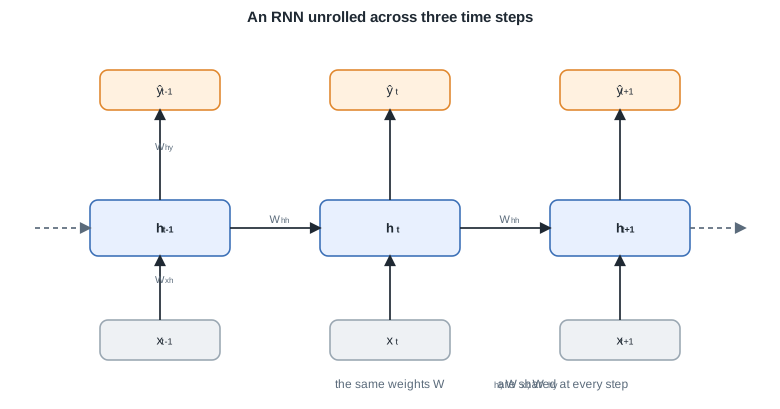
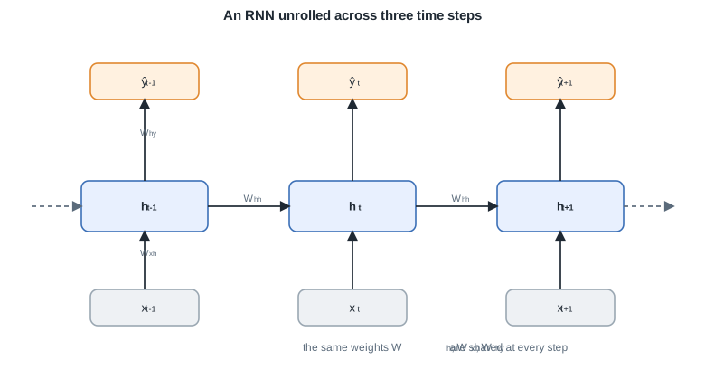
| + | ## 12.3 Unrolling in time |
| Because the same cell is reused, we can **unroll** the recurrence into a chain: draw one copy of the cell per time step and connect the hidden state of each copy to the next. The unrolled view is an ordinary feedforward graph (with tied weights), which is exactly what makes gradient computation possible. | |
| - |  |
| + |  |
| *Unrolled in time, a recurrent network reuses the same weights at every step and passes the hidden state forward.* | |
| *Remark:* the horizontal arrows between hidden states are the only path along which information from the past reaches the present. Every one of them multiplies by the same matrix $W_{hh}$, which is the source of both the model's power and its training difficulty. | |
| - | ## 13.4 Backpropagation through time |
| + | ## 12.4 Backpropagation through time |
| Training minimizes a total cost that sums the per-step loss over the sequence. With per-step loss $L_t$ comparing $\hat{y}_t$ to the target $y_t$, the cost for one sequence is: | |
| @@ 74,7 74,7 @@ | |
| *Remark:* in practice the sum over $k$ is cut off after a fixed window, which is called truncated BPTT. It bounds memory and compute per update at the cost of ignoring dependencies longer than the window. | |
| - | ## 13.5 Vanishing and exploding gradients |
| + | ## 12.5 Vanishing and exploding gradients |
| The inner product $\prod_{i=k+1}^{t} \frac{\partial h_i}{\partial h_{i-1}}$ is what carries gradient information from step $t$ back to step $k$. From the recurrence $h_i = g(W_{hh} h_{i-1} + W_{xh} x_i + b_h)$, each factor is: | |
| @@ 86,7 86,7 @@ | |
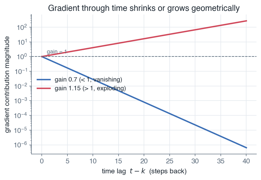
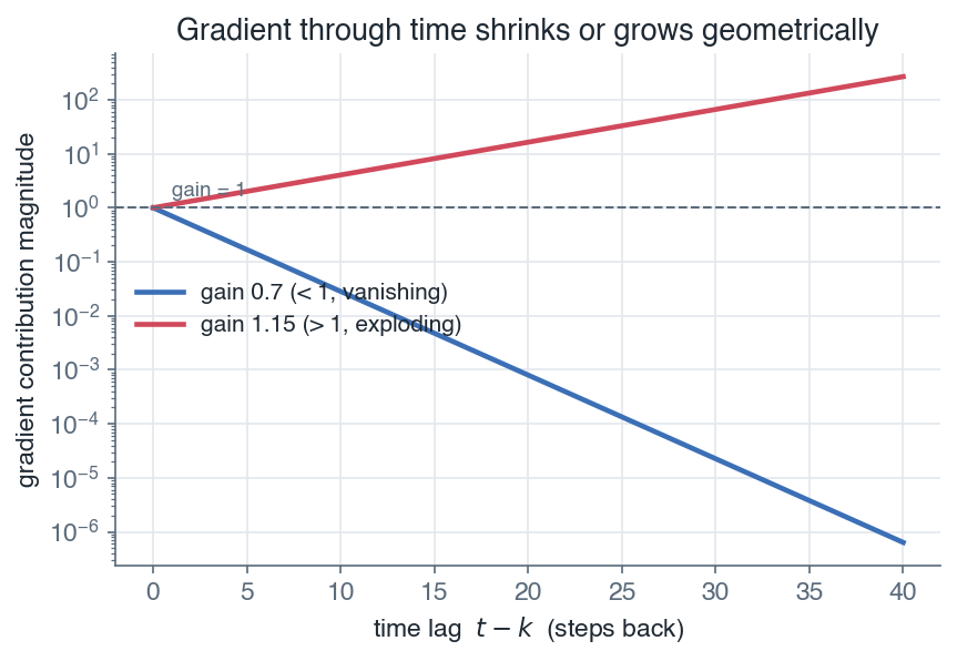
| This product of $t - k$ near-identical factors behaves roughly like a matrix raised to the power $t - k$. If the relevant magnitude (informally, the largest singular value of $\operatorname{diag}(g'(z_i)) W_{hh}$) is below $1$, the product shrinks geometrically toward zero as the gap grows, so distant gradients **vanish**. If it is above $1$, the product blows up and gradients **explode**. | |
| - |  |
| + |  |
| *Through many time steps the gradient shrinks or grows geometrically, so long-range dependencies are hard for a plain RNN to learn.* | |
| @@ 103,4 103,4 @@ | |
| *The next lesson introduces the LSTM and GRU, gated architectures that carry a cell state through additive updates so gradients can travel across long spans without vanishing.* | |
| --- | |
| - | Next: [LSTM and GRU](/en/Deep%20Learning/14%20LSTM%20and%20GRU) · [Course overview](/en/Deep%20Learning) |
| + | Next: [LSTM and GRU](/en/Deep%20Learning/13%20LSTM%20and%20GRU) · [Course overview](/en/Deep%20Learning) |
| en/Deep Learning/13 Recurrent networks/bptt-decay.png .. en/Deep Learning/12 Recurrent networks/bptt-decay.png | |
| en/Deep Learning/13 Recurrent networks/rnn-unrolled.svg .. en/Deep Learning/12 Recurrent networks/rnn-unrolled.svg | |
| en/Deep Learning/14 LSTM and GRU.md .. en/Deep Learning/13 LSTM and GRU.md | |
| @@ 1,4 1,4 @@ | |
| - | # 14. LSTM and GRU |
| + | # 13. LSTM and GRU |
| A plain recurrent network struggles to carry information across many time steps because repeated multiplication by the same weight matrix makes gradients vanish or explode. Gated recurrent cells fix this by adding a state that flows through time with mostly additive updates, controlled by learned gates. This module builds the long short-term memory (LSTM) cell and the lighter gated recurrent unit (GRU), and contrasts when to reach for each. | |
| @@ 9,7 9,7 @@ | |
| - Write the GRU reset and update gates and its interpolated hidden state. | |
| - Compare LSTM and GRU on gate count, cell state, parameter count, and typical use. | |
| - | ## 14.1 The gating idea |
| + | ## 13.1 The gating idea |
| A vanilla recurrent layer updates its hidden state by $h_t = g(W_h h_{t-1} + W_x x_t + b)$. Backpropagating the loss through $T$ steps multiplies many Jacobians of this map together, so the gradient magnitude scales roughly like the $T$-th power of the recurrent weight's spectral radius. Below one it vanishes, above one it explodes, and in both cases the network cannot learn dependencies that span many steps. | |
| @@ 17,11 17,11 @@ | |
| *Remark:* the key word is additive. Multiplicative recurrence compounds a factor at every step, while an additive path lets the state persist by default and change only when a gate opens. | |
| - | ## 14.2 The LSTM cell |
| + | ## 13.2 The LSTM cell |
| Throughout, $[h_{t-1}, x_t]$ denotes the concatenation of the previous hidden state and the current input into one vector. Each gate is a vector in $(0, 1)$ produced by a sigmoid $\sigma$ applied to an affine map of that concatenation, so a gate value near $1$ lets information through and a value near $0$ blocks it. | |
| - | ### 14.2.1 The three gates |
| + | ### 13.2.1 The three gates |
| The **forget** gate $f_t$ decides how much of the old cell state to keep, the **input** gate $i_t$ decides how much of the new candidate to write, and the **output** gate $o_t$ decides how much of the cell state to expose as the hidden state: | |
| @@ 29,7 29,7 @@ | |
| *Remark:* the gates share the same functional form and differ only in their learned parameters. The bias is explicit here, exactly as with the feedforward layers of earlier modules, and is never folded into the weight matrix. | |
| - | ### 14.2.2 Candidate and cell update |
| + | ### 13.2.2 Candidate and cell update |
| A $\tanh$ layer proposes a **candidate** update $\tilde{c}_t$, the new content the cell could store: | |
| @@ 41,7 41,7 @@ | |
| When $f_t \approx 1$ and $i_t \approx 0$ the cell simply copies $c_{t-1}$, which is the constant error carousel: $\partial c_t / \partial c_{t-1} \approx \mathrm{diag}(f_t)$, so gradients pass through nearly unattenuated. | |
| - | ### 14.2.3 Hidden state |
| + | ### 13.2.3 Hidden state |
| The hidden state is the squashed cell state, gated by the output gate: | |
| @@ 49,21 49,21 @@ | |
| *Remark:* the cell state $c_t$ is the long-term memory that flows along the carousel, while the hidden state $h_t$ is the filtered view exposed to the next layer and to the output at this step. Keeping them separate is what distinguishes the LSTM from the GRU below. | |
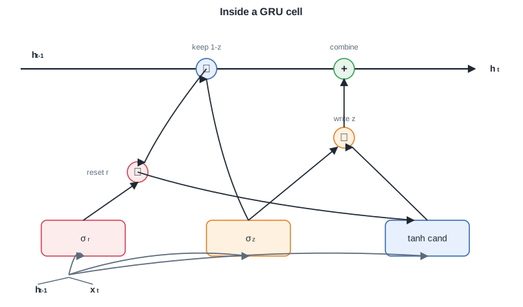
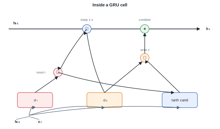
| - | ## 14.3 The GRU |
| + | ## 13.3 The GRU |
| The GRU merges the cell and hidden state into a single $h_t$ and uses only two gates, so it has fewer parameters while keeping the additive-update benefit. | |
| - |  |
| + |  |
| *The GRU merges the cell and hidden state and uses just a reset and an update gate.* | |
| - | ### 14.3.1 Reset and update gates |
| + | ### 13.3.1 Reset and update gates |
| The **reset** gate $r_t$ controls how much past state feeds the candidate, and the **update** gate $z_t$ controls how much of the state to refresh: | |
| $$\boxed{ r_t = \sigma\!\left(W_r\,[h_{t-1}, x_t] + b_r\right), \quad z_t = \sigma\!\left(W_z\,[h_{t-1}, x_t] + b_z\right) }$$ | |
| - | ### 14.3.2 Candidate and interpolated state |
| + | ### 13.3.2 Candidate and interpolated state |
| The candidate uses a reset-gated version of the previous hidden state, and the new state is a gated interpolation between the old state and the candidate: | |
| @@ 71,7 71,7 @@ | |
| *Remark:* the interpolation form ties the keep and write fractions together with a single gate: whatever weight $z_t$ gives the candidate, $1 - z_t$ is left for the past. The LSTM sets its keep fraction $f_t$ and write fraction $i_t$ independently, which is one more gate and one more matrix. | |
| - | ## 14.4 LSTM versus GRU |
| + | ## 13.4 LSTM versus GRU |
| Both cells solve the vanishing-gradient problem with an additive state path. They differ in how many gates carry that path and whether the long-term memory is kept separate from the exposed state. | |
| @@ 85,11 85,11 @@ | |
| *Remark:* in practice the two often reach comparable accuracy. The GRU trains faster and generalizes well on smaller datasets, while the extra capacity of the LSTM can help on very long sequences. Treat the choice as a tunable hyperparameter rather than a settled rule. | |
| - | ## 14.5 Anatomy of a gated cell |
| + | ## 13.5 Anatomy of a gated cell |
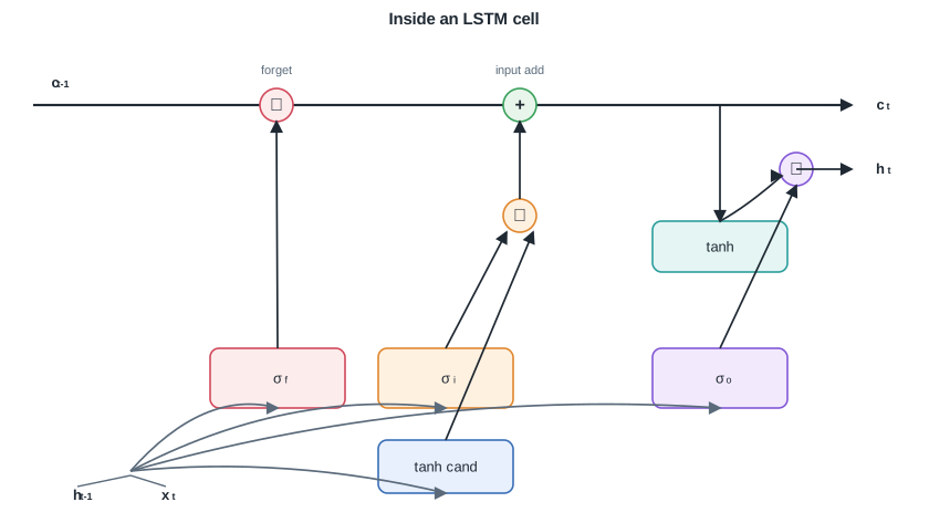
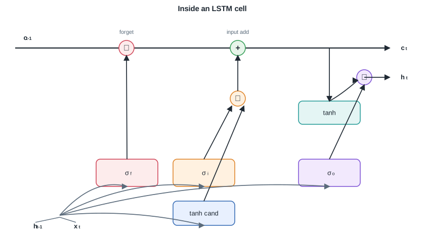
| The diagram traces one LSTM step: the previous cell state enters on the additive path, the gates modulate what is forgotten, written, and exposed, and the outputs feed the next step. | |
| - |  |
| + |  |
| *The LSTM cell carries a cell state along the top, edited by a forget multiply and an input add, with sigmoid gates controlling the flow.* | |
| @@ 98,4 98,4 @@ | |
| *Gates let a recurrent state persist over long spans, but they still read one step at a time. The next part lets every position attend directly to every other, removing the sequential bottleneck.* | |
| --- | |
| - | Next: [Attention](/en/Deep%20Learning/15%20Attention) · [Course overview](/en/Deep%20Learning) |
| + | Next: [Attention](/en/Deep%20Learning/14%20Attention) · [Course overview](/en/Deep%20Learning) |
| en/Deep Learning/14 LSTM and GRU/gru-cell.svg .. en/Deep Learning/13 LSTM and GRU/gru-cell.svg | |
| en/Deep Learning/14 LSTM and GRU/lstm-cell.svg .. en/Deep Learning/13 LSTM and GRU/lstm-cell.svg | |
| en/Deep Learning/15 Attention.md .. en/Deep Learning/14 Attention.md | |
| @@ 1,4 1,4 @@ | |
| - | # 15. Attention |
| + | # 14. Attention |
| Recurrent encoder-decoder models push a whole input sequence through a single fixed context vector, which caps how much they can remember for long inputs. Attention removes that bottleneck by letting the decoder read every encoder state directly, weighting each one by how relevant it is to the current output step. This lesson builds the mechanism from alignment scores to the query-key-value view, which is the foundation the Transformer will generalize. | |
| @@ 9,7 9,7 @@ | |
| - Recast attention as a query attending over keys and values. | |
| - Connect this framing to self-attention and the Transformer. | |
| - | ## 15.1 The seq2seq bottleneck |
| + | ## 14.1 The seq2seq bottleneck |
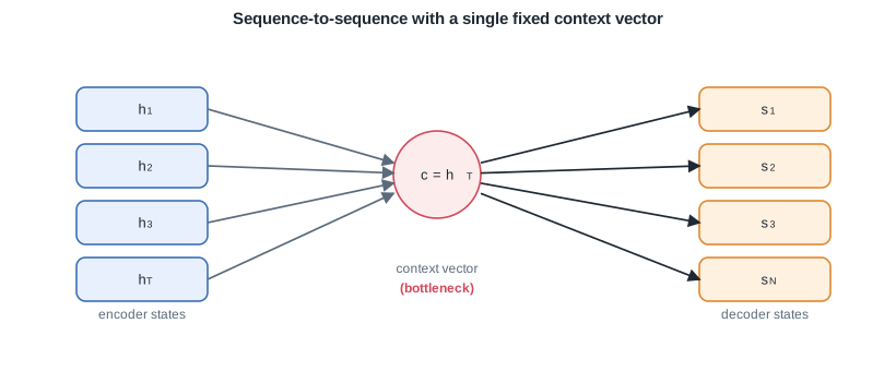
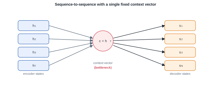
| A sequence-to-sequence model uses an encoder recurrent network to read the input tokens $x_1, \dots, x_T$ into hidden states $h_1, \dots, h_T$, then a decoder recurrent network to emit the output tokens. In the vanilla design the decoder is initialised from a single context vector, the encoder's last hidden state: | |
| @@ 19,21 19,21 @@ | |
| *Remark:* this is a genuine information bottleneck. For a short sentence $h_T$ can hold enough, but as $T$ grows the early tokens are overwritten and translation or summarisation quality drops sharply on long inputs. | |
| - |  |
| + |  |
| *Plain sequence-to-sequence squeezes the whole input into one fixed context vector, a bottleneck for long sequences.* | |
| The fix is to keep all encoder states $h_1, \dots, h_T$ available and let the decoder decide, at each step, which of them to read. | |
| - | ## 15.2 The attention mechanism |
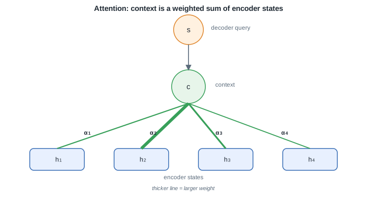
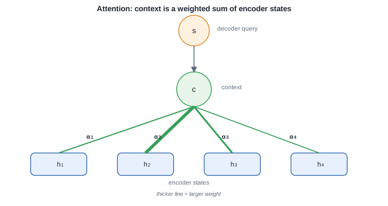
| + | ## 14.2 The attention mechanism |
| Instead of one context vector shared across all steps, attention builds a fresh context vector $c_i$ for each decoder step $i$. It does this in three stages: score, normalise, combine. | |
| - |  |
| + |  |
| *Attention scores each encoder state against the decoder query, then forms the context as a weighted sum of all states.* | |
| - | ### 15.2.1 Alignment scores |
| + | ### 14.2.1 Alignment scores |
| For decoder step $i$ with state $s_i$, a score function measures how well that state aligns with each encoder state $h_j$: | |
| @@ 43,7 43,7 @@ | |
| *Remark:* $s_i$ is usually the decoder state just before emitting token $i$, so the model chooses what to look at using what it has produced so far. | |
| - | ### 15.2.2 Attention weights |
| + | ### 14.2.2 Attention weights |
| The scores are turned into a probability distribution over input positions with a softmax across $j$: | |
| @@ 51,7 51,7 @@ | |
| Each $\alpha_{i,j} \in (0,1)$ and $\sum_j \alpha_{i,j} = 1$, so the weights say how much of the decoder's attention at step $i$ goes to input position $j$. | |
| - | ### 15.2.3 Context vector |
| + | ### 14.2.3 Context vector |
| The context vector for step $i$ is the weighted average of the encoder states, using the attention weights: | |
| @@ 61,11 61,11 @@ | |
| *Remark:* because every step averages over all $h_j$, no single fixed vector has to carry the whole input. The bottleneck of 15.1 is gone, and long inputs no longer degrade so quickly. | |
| - | ## 15.3 Score functions |
| + | ## 14.3 Score functions |
| The score function in 15.2.1 is a design choice. Two forms dominate the early attention literature. | |
| - | ### 15.3.1 Additive (Bahdanau) score |
| + | ### 14.3.1 Additive (Bahdanau) score |
| The additive score, from Bahdanau and co-authors, feeds the two states through a small one-hidden-layer network with learned matrices $W_1$ and $W_2$ and a learned vector $v$: | |
| @@ 73,7 73,7 @@ | |
| It works even when $s_i$ and $h_j$ have different dimensions, since $W_1$ and $W_2$ project both into a shared space before the $\tanh$. | |
| - | ### 15.3.2 Multiplicative (Luong) score |
| + | ### 14.3.2 Multiplicative (Luong) score |
| The multiplicative score, from Luong and co-authors, is a plain dot product between the two states: | |
| @@ 81,7 81,7 @@ | |
| It has no extra parameters in its simplest form and is far cheaper to compute, since a whole matrix of scores is a single matrix multiplication. A general variant inserts a learned matrix $W$ as $s_i^{\top} W h_j$ to handle mismatched dimensions. | |
| - | ### 15.3.3 Which to use |
| + | ### 14.3.3 Which to use |
| | Aspect | Additive (Bahdanau) | Multiplicative (Luong) | | |
| | --- | --- | --- | | |
| @@ 93,11 93,11 @@ | |
| *Remark:* the dot product grows with the dimension of the states, so at large widths its variance gets big and pushes the softmax into flat regions. Scaling the score by $1/\sqrt{d}$ fixes this, and that scaled dot product is exactly what the Transformer will adopt. | |
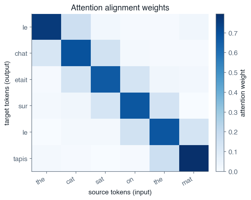
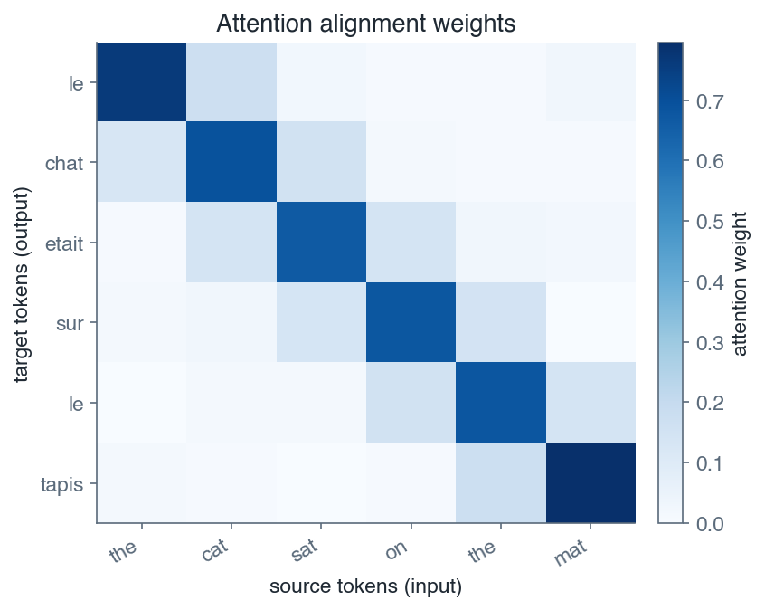
| - | ## 15.4 Query, key, value |
| + | ## 14.4 Query, key, value |
| Attention has a cleaner reading that drops the encoder-decoder framing. Rename the pieces: the state that does the looking is a query, and each thing that can be looked at contributes a key (used for scoring) and a value (used in the sum). | |
| - |  |
| + |  |
| *An attention weight matrix: each output token draws mostly from a few input tokens.* | |
| @@ 114,4 114,4 @@ | |
| *Building the query, key, and value from one sequence with learned projections turns attention into a general sequence layer, which is exactly where the next lesson on Transformers begins.* | |
| --- | |
| - | Next: [Transformers](/en/Deep%20Learning/16%20Transformers) · [Course overview](/en/Deep%20Learning) |
| + | Next: [Transformers](/en/Deep%20Learning/15%20Transformers) · [Course overview](/en/Deep%20Learning) |
| en/Deep Learning/15 Attention/attention-heatmap.png .. en/Deep Learning/14 Attention/attention-heatmap.png | |
| en/Deep Learning/15 Attention/attention-weights.svg .. en/Deep Learning/14 Attention/attention-weights.svg | |
| en/Deep Learning/15 Attention/seq2seq-bottleneck.svg .. en/Deep Learning/14 Attention/seq2seq-bottleneck.svg | |
| en/Deep Learning/16 Transformers.md .. en/Deep Learning/15 Transformers.md | |
| @@ 1,4 1,4 @@ | |
| - | # 16. Transformers |
| + | # 15. Transformers |
| The Transformer replaces recurrence with attention alone. It processes a whole sequence of token embeddings in parallel, letting every token attend to every other token through learned queries, keys, and values. This lesson builds the architecture from self-attention, assuming embeddings (lesson 12) and the attention mechanism (lesson 15), and reuses normalization (lesson 8) and residual connections (lesson 11). | |
| @@ 10,7 10,7 @@ | |
| - Assemble a Transformer block from residual connections and layer normalization. | |
| - Place the block inside the encoder-decoder stack and name its encoder-only and decoder-only variants. | |
| - | ## 16.1 Self-attention and Q, K, V |
| + | ## 15.1 Self-attention and Q, K, V |
| A sequence of $n$ tokens is represented by an embedding matrix $X \in \mathbb{R}^{n \times d}$, one row per token. Self-attention lets each token gather information from the others by asking a question (a query), matching it against every token's label (a key), and reading out content (a value). | |
| @@ 20,7 20,7 @@ | |
| *Remark:* the projections are the only learned parameters here, and the same three matrices are shared across all positions. Because a token is compared against every other token, the operation captures long-range dependencies in a single step, unlike a recurrence that must carry information forward one position at a time. | |
| - | ## 16.2 Scaled dot-product attention |
| + | ## 15.2 Scaled dot-product attention |
| Each query is compared against every key by a dot product, giving an $n \times n$ matrix of raw scores. The scores are scaled, turned into weights by a row-wise softmax, and used to average the values: | |
| @@ 28,7 28,7 @@ | |
| Row $i$ of the softmax is a probability distribution over all tokens, so output row $i$ is a weighted average of the value vectors, weighted by how relevant each token is to token $i$. | |
| - | ### 16.2.1 Why divide by $\sqrt{d_k}$ |
| + | ### 15.2.1 Why divide by $\sqrt{d_k}$ |
| If the entries of $q$ and $k$ are independent with zero mean and unit variance, the dot product $q^{T} k = \sum_{j=1}^{d_k} q_j k_j$ has variance $d_k$, so its typical magnitude grows like $\sqrt{d_k}$. | |
| @@ 36,7 36,7 @@ | |
| Large scores push the softmax into a saturated regime where one weight is near $1$ and the rest are near $0$, and the softmax gradient there is tiny. Dividing by $\sqrt{d_k}$ keeps the logits at a moderate scale, which keeps the softmax gradients healthy and stabilizes training. | |
| - | ## 16.3 Multi-head attention |
| + | ## 15.3 Multi-head attention |
| A single attention computation forces every relationship to be read through one $d_k$-dimensional subspace. Multi-head attention runs $h$ attention operations in parallel, each with its own projections, so different heads can specialize (one on syntax, another on coreference, and so on). | |
| @@ 50,7 50,7 @@ | |
| *Remark:* the per-head width is usually set to $d_k = d_v = d / h$, so the concatenation returns to width $d$ and the total cost matches a single full-width head. The heads are independent and computed in parallel, which is one reason Transformers train efficiently on modern hardware. | |
| - | ## 16.4 Positional encoding |
| + | ## 15.4 Positional encoding |
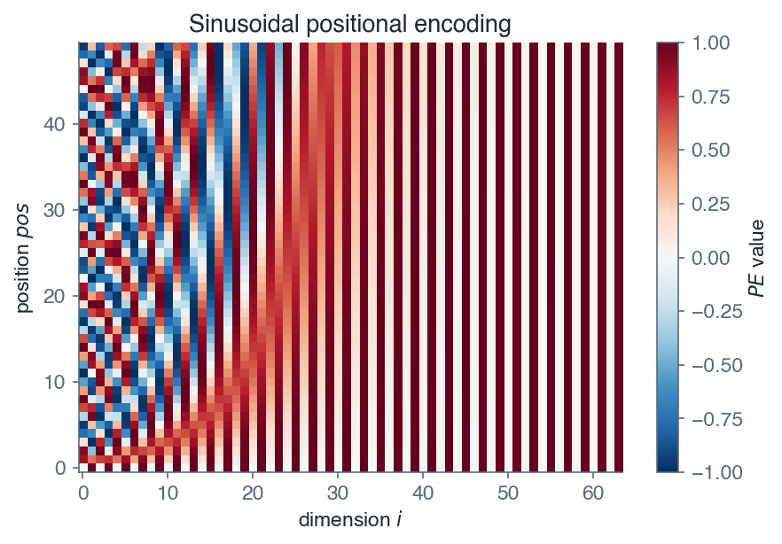
| Attention treats its input as a set: permuting the rows of $X$ permutes the output the same way, so the operation is order-agnostic. Language is not, therefore position must be supplied explicitly. The original Transformer adds a fixed sinusoidal encoding to the embeddings, using a different frequency per feature dimension: | |
| @@ 58,19 58,19 @@ | |
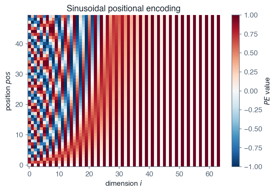
| Here $pos$ is the token position and $i$ indexes the feature dimension. Low dimensions vary quickly with position and high dimensions vary slowly, so the vector encodes position across many scales. The encoding is added to the token embedding before the first block. | |
| - |  |
| + |  |
| *Sinusoidal positional encodings vary quickly in low dimensions and slowly in high dimensions, giving each position a unique multi-scale signature.* | |
| *Remark:* sinusoids let a relative shift $PE_{pos+k}$ be written as a linear function of $PE_{pos}$, so the model can learn to attend by relative offset. The encodings are fixed (not learned) and extend to sequence lengths unseen during training. Many later models replace them with learned or relative position schemes. | |
| - | ## 16.5 The Transformer block |
| + | ## 15.5 The Transformer block |
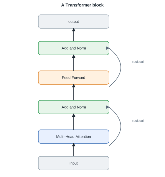
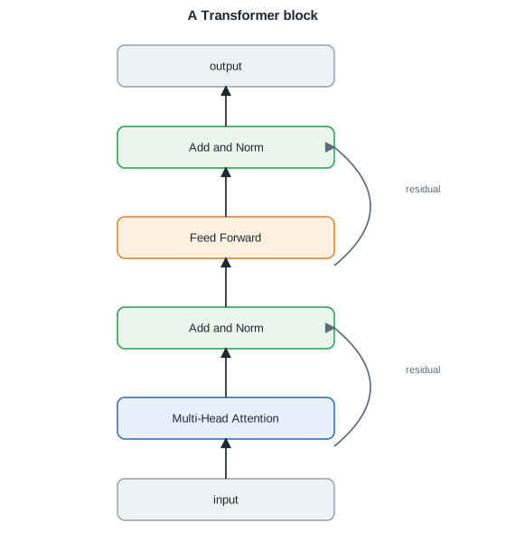
| Each sublayer is wrapped in a residual connection followed by layer normalization, which keeps gradients flowing through deep stacks and stabilizes the activation scale: | |
| $$\boxed{ x \leftarrow \mathrm{LayerNorm}\!\left(x + \mathrm{Sublayer}(x)\right) }$$ | |
| - |  |
| + |  |
| *A Transformer block wraps multi-head attention and a feed-forward network, each in a residual connection followed by layer normalization.* | |
| @@ 89,15 89,15 @@ | |
| | Residual connection | preserve a gradient path | the depth | | |
| | Layer normalization | stabilize the activation scale | the features per token | | |
| - | ## 16.6 The encoder-decoder architecture |
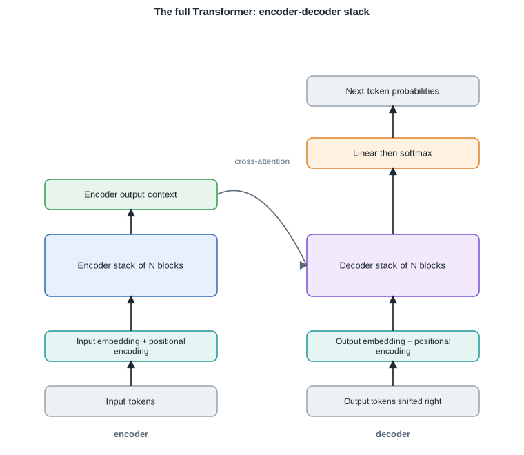
| + | ## 15.6 The encoder-decoder architecture |
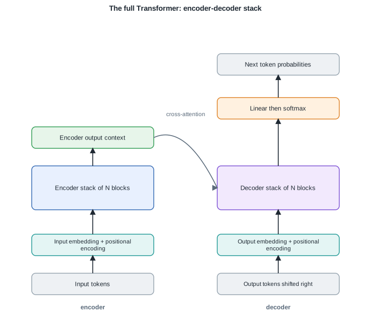
| The full Transformer stacks $N$ identical blocks in an encoder and $N$ in a decoder. The encoder maps the input sequence to a set of context vectors. Each decoder block has three sublayers: masked self-attention over the tokens generated so far (the mask blocks attention to future positions), cross-attention whose queries come from the decoder and whose keys and values come from the encoder output, and a feed-forward network. A final linear layer plus softmax turns the top decoder states into a distribution over the vocabulary. | |
| - |  |
| + |  |
| *The full Transformer: a stack of encoder blocks and a stack of decoder blocks joined by cross-attention.* | |
| - | ### 16.6.1 Variants |
| + | ### 15.6.1 Variants |
| Not every task needs both halves. Two families dominate practice: | |
| en/Deep Learning/16 Transformers/positional-encoding.png .. en/Deep Learning/15 Transformers/positional-encoding.png | |
| en/Deep Learning/16 Transformers/transformer-block.svg .. en/Deep Learning/15 Transformers/transformer-block.svg | |
| en/Deep Learning/16 Transformers/transformer-stack.svg .. en/Deep Learning/15 Transformers/transformer-stack.svg | |
| en/Machine Learning/01 Introduction.md .. | |
| @@ 1,15 1,6 @@ | |
| # 1. Introduction | |
| - | Machine learning builds models that learn patterns from data instead of being explicitly programmed with rules. This module fixes the notation used throughout the course and maps the landscape of problems and models, so later modules can stay terse and formula-first. |
| - | |
| - | **Objectives** |
| - | - Distinguish supervised, unsupervised, and reinforcement learning by their feedback signal. |
| - | - Situate the stages of a machine learning project and its feedback loops. |
| - | - Fix the notation used across the whole course. |
| - | - Define the training set, the hypothesis, and the design matrix. |
| - | - Adopt the intercept convention $x_0 = 1$. |
| - | - Classify a supervised problem by the type of its output. |
| - | - Distinguish discriminative from generative models. |
| + | Machine learning builds models that learn patterns from data instead of being explicitly programmed with rules. This module fixes the notation used throughout the course and maps the kinds of problems it tackles, so later modules can stay terse and formula-first. |
| ## 1.1 Types of learning | |
| @@ 33,25 24,9 @@ | |
| *Remark:* the boundaries are not rigid. Semi-supervised learning mixes a few labelled examples with many unlabelled ones, and self-supervised learning manufactures labels from the data itself, for example by hiding a word and predicting it. Both reuse the supervised machinery introduced in this course. | |
| - | ## 1.2 The workflow |
| - | |
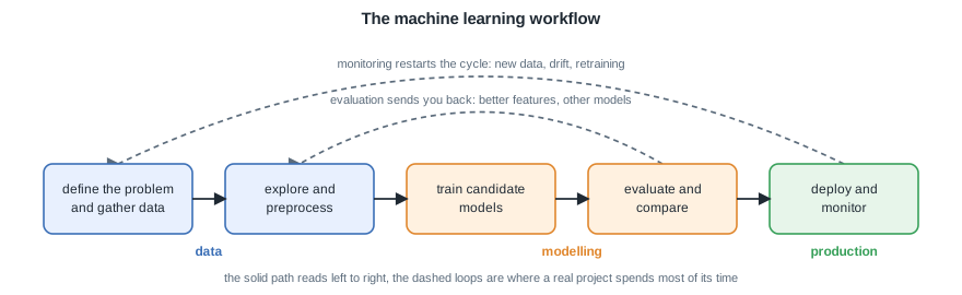
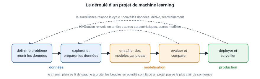
| - | A machine learning project is not a straight line from data to model. It runs as a loop: every evaluation reveals something that sends the work back to an earlier stage, and once deployed, a model faces new data that eventually restarts the cycle. |
| - | |
| - |  |
| - | |
| - | *The solid path is the nominal order. The dashed arrows are where real projects spend most of their time: reworking features and models after evaluation, and retraining after monitoring.* |
| - | |
| - | 1. **Define the problem and gather data.** Turn the question into a prediction task by fixing the input $x$, the target $y$, and the metric that counts as success. The choices made here bound everything downstream, because no model can recover information the data does not contain. |
| - | 2. **Explore and preprocess the data.** Inspect distributions, missing values, and outliers, then clean, encode, and scale the features. Set aside a test set before tuning anything against it, so the final performance estimate stays honest. |
| - | 3. **Train candidate models.** Start with a simple baseline, then fit richer families by minimizing a loss over the parameters $\theta$ ([General concepts](/en/Machine%20Learning/02%20General%20concepts)). |
| - | 4. **Evaluate and compare.** Measure each candidate on data it has never seen, with validation and cross-validation ([General concepts](/en/Machine%20Learning/02%20General%20concepts)) and a metric matched to the problem. The verdict usually points back to step 2 or 3: better features, another model family, or more data. |
| - | 5. **Deploy and monitor.** In production the incoming data drifts away from the training distribution, so performance must be watched and retraining planned. That discipline has its own course: [MLOps](/en/MLOps). |
| + | ## 1.2 The course notation |
| - | *Remark:* in practice most of the effort goes into steps 1, 2, and 4. Training itself is often the cheapest step, and the ceiling on model quality is set by the data. |
| - | |
| - | ## 1.3 Notation and setup |
| - | |
| - | ### 1.3.1 Training set |
| + | ### 1.2.1 Training set |
| The training set is defined as a collection of $m$ labelled examples: | |
| @@ 66,21 41,21 @@ | |
| *Remark:* the superscript $(i)$ indexes the example and the subscript $j$ indexes the feature, so $x_j^{(i)}$ is feature $j$ of example $i$. | |
| - | By convention the input is augmented with a constant intercept term $x_0 = 1$, so $x \in \mathbb{R}^{n+1}$ and the parameters are $\theta \in \mathbb{R}^{n+1}$. |
| + | By convention the input is augmented with a constant intercept term $x_0 = 1$, so $x \in \mathbb{R}^{n+1}$ and the parameters are $w \in \mathbb{R}^{n+1}$. |
| - | $$\boxed{ x_0 = 1, \quad x \in \mathbb{R}^{n+1}, \quad \theta \in \mathbb{R}^{n+1} }$$ |
| + | $$\boxed{ x_0 = 1, \quad x \in \mathbb{R}^{n+1}, \quad w \in \mathbb{R}^{n+1} }$$ |
| - | *Remark:* the intercept lets a single dot product $\theta^T x$ carry the bias term, so no separate constant has to be written. |
| + | *Remark:* the intercept lets a single dot product $w^T x$ carry the bias term, so no separate constant has to be written. |
| - | ### 1.3.2 Hypothesis |
| + | ### 1.2.2 Hypothesis |
| A hypothesis is defined as a function chosen from a model family that maps an input to a prediction: | |
| - | $$\boxed{ h_\theta : x \mapsto h_\theta(x) }$$ |
| + | $$\boxed{ h_w : x \mapsto \hat{y} = h_w(x) }$$ |
| - | Learning is the search, over the parameters $\theta$, for the hypothesis that best fits the training set. |
| + | Two notations, two roles: $h_w$ names the function, and $\hat{y}$ names the value it predicts for one input, the hat marking an estimate of the label $y$. Learning is the search, over the parameters $w$, for the hypothesis that best fits the training set. |
| - | ### 1.3.3 Design matrix |
| + | ### 1.2.3 Design matrix |
| The design matrix stacks the $m$ transposed inputs row by row, and the target vector collects the labels: | |
| @@ 88,11 63,9 @@ | |
| Here $X \in \mathbb{R}^{m \times (n+1)}$ (each augmented input is a row) and $y \in \mathbb{R}^{m}$. | |
| - | *Remark:* with this layout many models reduce to compact matrix expressions, for example a linear prediction over all examples is $X\theta$. |
| + | *Remark:* with this layout many models reduce to compact matrix expressions, for example a linear prediction over all examples is $Xw$. |
| - | ## 1.4 Types of problems and models |
| - | |
| - | ### 1.4.1 Type of prediction |
| + | ## 1.3 Types of problems |
| A supervised problem is named by the nature of its target $y$. | |
| @@ 107,34 80,6 @@ | |
| *Left: regression fits a continuous output. Right: classification separates the input space into classes.* | |
| - | ### 1.4.2 Type of model |
| - | |
| - | A model is discriminative if it learns the conditional $p(y \mid x)$ directly, and generative if it models how the data are generated, $p(x \mid y)$ and $p(y)$, then inverts via Bayes' rule: |
| - | |
| - | $$\boxed{ p(y \mid x) = \frac{p(x \mid y)\, p(y)}{p(x)} }$$ |
| - | |
| - | | Aspect | Discriminative | Generative | |
| - | | --- | --- | --- | |
| - | | Goal | model the boundary between classes | model how each class generates data | |
| - | | What is learned | $p(y \mid x)$ directly | $p(x \mid y)$ and $p(y)$, then Bayes | |
| - | | Examples | logistic regression, SVM | Gaussian discriminant analysis, naive Bayes | |
| - | |
| - | *Remark:* $p(x)$ is the same for every class, so for classification it can be dropped and the most probable class taken via $\arg\max_y\, p(x \mid y)\, p(y)$. |
| - | |
| - | ### 1.4.3 Putting it together |
| - | |
| - | The output type fixes regression vs classification, and the modelling choice fixes discriminative vs generative. Together they select a model family. |
| - | |
| - | ```mermaid |
| - | graph TD |
| - | A["supervised problem"] --> B{"output type?"} |
| - | B -->|"continuous"| C["regression"] |
| - | B -->|"discrete"| D["classification"] |
| - | D --> E{"model type?"} |
| - | E -->|"discriminative"| F["logistic regression, SVM"] |
| - | E -->|"generative"| G["GDA, naive Bayes"] |
| - | ``` |
| - | |
| *With the problem framed and the notation fixed, the next part turns to what learning really demands: minimizing a loss is easy, generalizing beyond the training set is the challenge.* | |
| --- | |
| en/Machine Learning/01 Introduction/ml-workflow.svg .. /dev/null | |
| @@ 1,40 0,0 @@ | |
| - | <svg xmlns="http://www.w3.org/2000/svg" viewBox="0 0 880 270" width="880" height="270" font-family="Helvetica, Arial, sans-serif"> |
| - | <defs> |
| - | <marker id="arrow" viewBox="0 0 10 10" refX="8.5" refY="5" markerWidth="7" markerHeight="7" orient="auto-start-reverse"><path d="M0 0L10 5L0 10z" fill="#1f2933"/></marker> |
| - | <marker id="arrowmuted" viewBox="0 0 10 10" refX="8.5" refY="5" markerWidth="7" markerHeight="7" orient="auto-start-reverse"><path d="M0 0L10 5L0 10z" fill="#5b6b7b"/></marker> |
| - | </defs> |
| - | <rect width="880" height="270" fill="#ffffff"/> |
| - | <text x="440" y="22" font-size="15" font-weight="600" fill="#1f2933" text-anchor="middle">The machine learning workflow</text> |
| - | |
| - | <path d="M772 150 Q440 -10 108 150" fill="none" stroke="#5b6b7b" stroke-width="1.7" stroke-dasharray="5 4" marker-end="url(#arrowmuted)"/> |
| - | <text x="440" y="62" font-size="11" fill="#5b6b7b" text-anchor="middle">monitoring restarts the cycle: new data, drift, retraining</text> |
| - | <path d="M606 150 Q440 55 274 150" fill="none" stroke="#5b6b7b" stroke-width="1.7" stroke-dasharray="5 4" marker-end="url(#arrowmuted)"/> |
| - | <text x="440" y="95" font-size="11" fill="#5b6b7b" text-anchor="middle">evaluation sends you back: better features, other models</text> |
| - | |
| - | <rect x="40" y="150" width="136" height="64" rx="8" fill="#e8f0fe" stroke="#3b6fb6" stroke-width="1.6"/> |
| - | <text x="108" y="177" font-size="12" fill="#1f2933" text-anchor="middle">define the problem</text> |
| - | <text x="108" y="194" font-size="12" fill="#1f2933" text-anchor="middle">and gather data</text> |
| - | <rect x="206" y="150" width="136" height="64" rx="8" fill="#e8f0fe" stroke="#3b6fb6" stroke-width="1.6"/> |
| - | <text x="274" y="177" font-size="12" fill="#1f2933" text-anchor="middle">explore and</text> |
| - | <text x="274" y="194" font-size="12" fill="#1f2933" text-anchor="middle">preprocess</text> |
| - | <rect x="372" y="150" width="136" height="64" rx="8" fill="#fff1e0" stroke="#e0872e" stroke-width="1.6"/> |
| - | <text x="440" y="177" font-size="12" fill="#1f2933" text-anchor="middle">train candidate</text> |
| - | <text x="440" y="194" font-size="12" fill="#1f2933" text-anchor="middle">models</text> |
| - | <rect x="538" y="150" width="136" height="64" rx="8" fill="#fff1e0" stroke="#e0872e" stroke-width="1.6"/> |
| - | <text x="606" y="177" font-size="12" fill="#1f2933" text-anchor="middle">evaluate and</text> |
| - | <text x="606" y="194" font-size="12" fill="#1f2933" text-anchor="middle">compare</text> |
| - | <rect x="704" y="150" width="136" height="64" rx="8" fill="#e7f5ea" stroke="#38a05a" stroke-width="1.6"/> |
| - | <text x="772" y="177" font-size="12" fill="#1f2933" text-anchor="middle">deploy and</text> |
| - | <text x="772" y="194" font-size="12" fill="#1f2933" text-anchor="middle">monitor</text> |
| - | |
| - | <line x1="176" y1="182" x2="206" y2="182" stroke="#1f2933" stroke-width="1.7" marker-end="url(#arrow)"/> |
| - | <line x1="342" y1="182" x2="372" y2="182" stroke="#1f2933" stroke-width="1.7" marker-end="url(#arrow)"/> |
| - | <line x1="508" y1="182" x2="538" y2="182" stroke="#1f2933" stroke-width="1.7" marker-end="url(#arrow)"/> |
| - | <line x1="674" y1="182" x2="704" y2="182" stroke="#1f2933" stroke-width="1.7" marker-end="url(#arrow)"/> |
| - | |
| - | <text x="191" y="234" font-size="12" font-weight="600" fill="#3b6fb6" text-anchor="middle">data</text> |
| - | <text x="523" y="234" font-size="12" font-weight="600" fill="#e0872e" text-anchor="middle">modelling</text> |
| - | <text x="772" y="234" font-size="12" font-weight="600" fill="#38a05a" text-anchor="middle">production</text> |
| - | |
| - | <text x="440" y="258" font-size="11" fill="#5b6b7b" text-anchor="middle">the solid path reads left to right, the dashed loops are where a real project spends most of its time</text> |
| - | </svg> |
| en/Machine Learning/02 General concepts.md .. | |
| @@ 2,18 2,9 @@ | |
| The introduction fixed the notation and named the learning paradigms. Before fitting any particular model, this module covers what learning actually means. Making a model fit the data it has seen is easy, making it perform on data it has never seen is the whole game. Polynomial regression serves as the running example, and the module closes with the reason geometric intuition fails in high dimension. | |
| - | **Objectives** |
| - | - Contrast supervised and unsupervised learning through what each one optimizes. |
| - | - Define a loss function and aggregate per-example losses into a cost to minimize. |
| - | - Fit polynomial regression and read its degree as a capacity knob. |
| - | - Distinguish training performance from generalization, and diagnose underfitting and overfitting. |
| - | - Control capacity continuously with a regularization penalty. |
| - | - Select hyperparameters with validation and cross-validation without contaminating the test set. |
| - | - State the curse of dimensionality and its consequences for learning. |
| - | |
| ## 2.1 Supervised versus unsupervised learning | |
| - | The [Introduction](/en/Machine%20Learning/01%20Introduction) named the paradigms by their feedback signal. Formally, supervised learning starts from labelled pairs $\{(x^{(i)}, y^{(i)})\}_{i=1}^{m}$ and searches a family of hypotheses for the $h_\theta$ whose predictions sit closest to the targets, closeness being measured by a loss function. Unsupervised learning has only the inputs $x^{(i)}$, so its objectives are built from the inputs alone: compact groups, informative directions, regions of high density. |
| + | The [Introduction](/en/Machine%20Learning/01%20Introduction) named the paradigms by their feedback signal. Formally, supervised learning starts from labelled pairs $\{(x^{(i)}, y^{(i)})\}_{i=1}^{m}$ and searches a family of hypotheses for the $h_w$ whose predictions sit closest to the targets, closeness being measured by a loss function. Unsupervised learning has only the inputs $x^{(i)}$, so its objectives are built from the inputs alone: compact groups, informative directions, regions of high density. |
| Everything in this module is stated for the supervised case, which occupies the rest of the course. The questions it answers (how well does this model generalize, how complex should it be, how do I choose between candidates) arise unchanged in the unsupervised setting. | |
| @@ 21,16 12,16 @@ | |
| ### 2.2.1 Loss function | |
| - | A loss function $L(z, y)$ is defined as a scalar penalty comparing a raw model score $z$ (or a predicted probability $\phi$) against the target $y$. Smaller is better. Each family of models is characterized by its loss. |
| + | A loss function $L(z, y)$ is defined as a scalar penalty comparing a raw model score $z$ (or a predicted probability $\hat{y}$) against the target $y$. Smaller is better. Each family of models is characterized by its loss. |
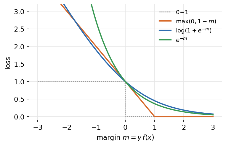
| | Loss | Formula $L(z,y)$ | Used by | | |
| | --- | --- | --- | | |
| | Least squared error | $\tfrac{1}{2}(y-z)^2$ | Linear regression | | |
| | Logistic | $\log\!\left(1+\exp(-yz)\right)$ | Logistic regression | | |
| | Hinge | $\max(0,\,1-yz)$ | SVM | | |
| - | | Cross-entropy | $-\left[\,y\log\phi+(1-y)\log(1-\phi)\,\right]$ | Neural networks | |
| + | | Cross-entropy | $-\left[\,y\log\hat{y}+(1-y)\log(1-\hat{y})\,\right]$ | Neural networks | |
| - | *Remark:* $z$ denotes a raw score such as $\theta^T x$, whereas $\phi \in (0,1)$ denotes a predicted probability. The cross-entropy row takes a probability $\phi$, not a raw score. |
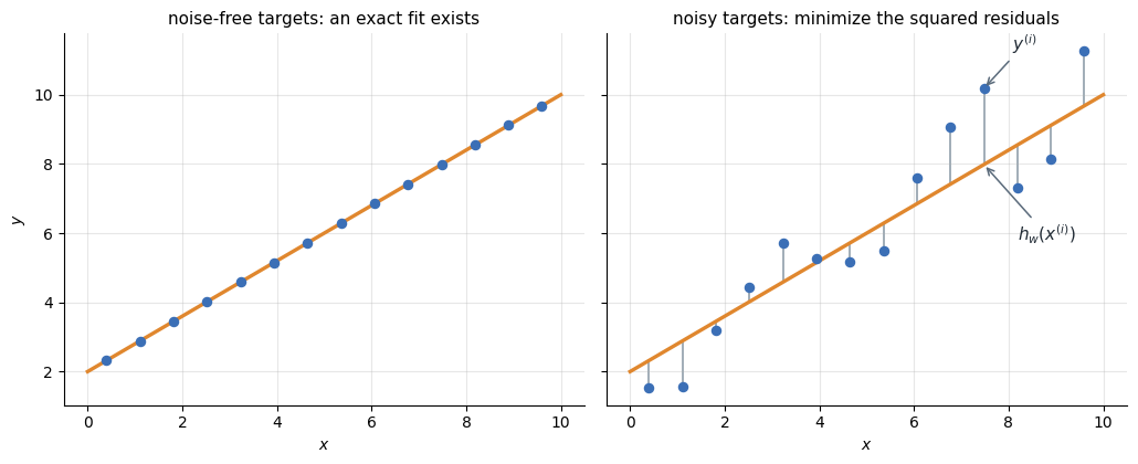
| + | *Remark:* $z$ denotes a raw score such as $w^T x$, whereas $\hat{y} \in (0,1)$ denotes a predicted probability, the model's estimate of the label $y$. The cross-entropy row takes a probability $\hat{y}$, not a raw score. |
|  | |
| @@ 38,11 29,11 @@ | |
| ### 2.2.2 Cost function | |
| - | The cost $J(\theta)$ is defined as the sum of the per-example losses over the whole training set of $m$ examples: |
| + | The cost $J(w)$ is defined as the sum of the per-example losses over the whole training set of $m$ examples: |
| - | $$\boxed{\,J(\theta)=\sum_{i=1}^{m} L\!\left(h_\theta(x^{(i)}),\,y^{(i)}\right)\,}$$ |
| + | $$\boxed{\,J(w)=\sum_{i=1}^{m} L\!\left(h_w(x^{(i)}),\,y^{(i)}\right)\,}$$ |
| - | Training a model means choosing $\theta$ to minimize $J(\theta)$. The algorithms that carry out this minimization (closed forms, gradient descent) arrive with the model modules. This module asks a different question: what does a low value of $J(\theta)$ actually prove? |
| + | Training a model means choosing $w$ to minimize $J(w)$. The algorithms that carry out this minimization (closed forms, gradient descent) arrive with the model modules. This module asks a different question: what does a low value of $J(w)$ actually prove? |
| *Remark:* the factor $\tfrac{1}{2}$ in the squared error is a convention that cancels with the exponent when differentiating, leaving a clean gradient. | |
| @@ 50,9 41,9 @@ | |
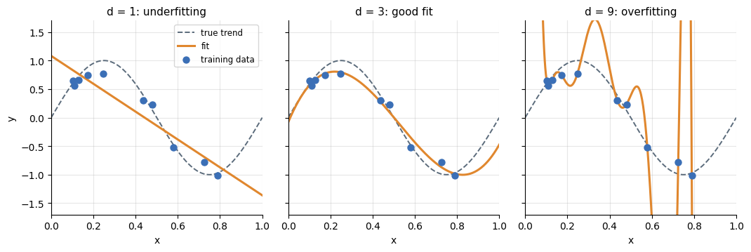
| To make everything concrete, take a single input $x$ and fit a polynomial of degree $d$ under the squared loss: | |
| - | $$\boxed{ h_\theta(x) = \theta^T \phi(x) = \sum_{j=0}^{d} \theta_j\, x^{j}, \qquad \phi(x) = (1, x, x^2, \dots, x^d) }$$ |
| + | $$\boxed{ h_w(x) = w^T \phi(x) = \sum_{j=0}^{d} w_j\, x^{j}, \qquad \phi(x) = (1, x, x^2, \dots, x^d) }$$ |
| - | The model stays linear in $\theta$, so least squares applies unchanged (the closed form is derived in [Linear regression](/en/Machine%20Learning/04%20Linear%20regression)). The degree $d$ is not fitted along with $\theta$: it is fixed before fitting and decides how flexible the curve is allowed to be. A knob of that kind, chosen rather than learned, is called a hyperparameter, and $d$ is our first one. |
| + | The model stays linear in $w$, so least squares applies unchanged (the closed form is derived in [Linear regression](/en/Machine%20Learning/04%20Linear%20regression)). The degree $d$ is not fitted along with $w$: it is fixed before fitting and decides how flexible the curve is allowed to be. A knob of that kind, chosen rather than learned, is called a hyperparameter, and $d$ is our first one. |
|  | |
| @@ 84,13 75,13 @@ | |
| ## 2.4 Regularization | |
| - | Choosing the degree is a coarse dial: capacity jumps by whole integers. A finer control keeps a flexible family but makes complexity expensive inside the cost itself, by adding a penalty $\Omega(\theta)$ scaled by a strength $\lambda \ge 0$: |
| + | Choosing the degree is a coarse dial: capacity jumps by whole integers. A finer control keeps a flexible family but makes complexity expensive inside the cost itself, by adding a penalty $\Omega(w)$ scaled by a strength $\lambda \ge 0$: |
| - | $$\boxed{\,J_\lambda(\theta)=\sum_{i=1}^{m} L\!\left(h_\theta(x^{(i)}),\,y^{(i)}\right) + \lambda\,\Omega(\theta)\,}$$ |
| + | $$\boxed{\,J_\lambda(w)=\sum_{i=1}^{m} L\!\left(h_w(x^{(i)}),\,y^{(i)}\right) + \lambda\,\Omega(w)\,}$$ |
| - | The classic choice is the squared norm $\Omega(\theta) = \lVert \theta \rVert_2^2$, the ridge penalty. The degree-9 fit only weaves through every point by using huge coefficients that cancel each other between the training points. The penalty makes those coefficients costly, so the minimizer trades a little training error for a much smoother curve. At $\lambda = 0$ the overfitted fit returns, as $\lambda \to \infty$ the curve flattens toward underfitting: $\lambda$ sweeps the same bias-variance dial as the degree, but continuously. |
| + | The classic choice is the squared norm $\Omega(w) = \lVert w \rVert_2^2$, the ridge penalty. The degree-9 fit only weaves through every point by using huge coefficients that cancel each other between the training points. The penalty makes those coefficients costly, so the minimizer trades a little training error for a much smoother curve. At $\lambda = 0$ the overfitted fit returns, as $\lambda \to \infty$ the curve flattens toward underfitting: $\lambda$ sweeps the same bias-variance dial as the degree, but continuously. |
| - | *Remark:* regularization does not decide the right complexity for you, it converts a discrete choice ($d$) into a continuous one ($\lambda$) that is easier to tune. $\lambda$ is a hyperparameter like the degree, chosen by the validation machinery of the next section. Where the penalty comes from (a prior on $\theta$, via maximum a posteriori) and what the L1 variant adds are the subjects of [Probabilistic formulation](/en/Machine%20Learning/03%20Probabilistic%20formulation) and [Linear regression](/en/Machine%20Learning/04%20Linear%20regression). |
| + | *Remark:* regularization does not decide the right complexity for you, it converts a discrete choice ($d$) into a continuous one ($\lambda$) that is easier to tune. $\lambda$ is a hyperparameter like the degree, chosen by the validation machinery of the next section. Where the penalty comes from (a prior on $w$, via maximum a posteriori) and what the L1 variant adds are the subjects of [Probabilistic formulation](/en/Machine%20Learning/03%20Probabilistic%20formulation) and [Linear regression](/en/Machine%20Learning/04%20Linear%20regression). |
| ## 2.5 Hyperparameters, validation, and cross-validation | |
| @@ 124,7 115,70 @@ | |
| *Remark:* choosing the winner on the test set inflates the estimate. With enough candidates one will look good by chance alone, the winner's curse, so selection and final evaluation must use different data. | |
| - | ## 2.6 Common validation pitfalls |
| + | ## 2.6 Regression metrics: how far off, on average |
| + | |
| + | The U-curve of section 2.3 already used a regression metric without naming it: the RMSE. For regression the raw material is the residual $y - \hat{y}$ between the label and the prediction $\hat{y} = h_w(x)$, and the metrics differ in how they aggregate the residuals, here for five predictions: |
| + | |
| + | | | $y$ | $\hat{y}$ | $y - \hat{y}$ | |
| + | | --- | --- | --- | --- | |
| + | | example 1 | 10 | 12 | $-2$ | |
| + | | example 2 | 14 | 13 | $1$ | |
| + | | example 3 | 8 | 9 | $-1$ | |
| + | | example 4 | 12 | 9 | $3$ | |
| + | | example 5 | 16 | 17 | $-1$ | |
| + | |
| + | | Metric | Formula | Here | Reads as | |
| + | | --- | --- | --- | --- | |
| + | | MSE | $\frac{1}{m}\sum_i \left(y^{(i)} - \hat{y}^{(i)}\right)^2$ | $3.2$ | the squared-error loss itself, in squared units | |
| + | | RMSE | $\sqrt{\text{MSE}}$ | $\approx 1.8$ | typical error, in the target's own units | |
| + | | MAE | $\frac{1}{m}\sum_i \left\lvert y^{(i)} - \hat{y}^{(i)} \right\rvert$ | $1.6$ | average miss, robust to outliers | |
| + | | $R^2$ | $1 - \sum_i \left(y^{(i)} - \hat{y}^{(i)}\right)^2 \big/ \sum_i \left(y^{(i)} - \bar{y}\right)^2$ | $0.6$ | variance explained, against predicting the mean | |
| + | |
| + | The mean here is $\bar{y} = 12$. Squaring makes the MSE and RMSE quadratic in each residual, so one large error dominates them, while the MAE grows only linearly: |
| + | |
| + | 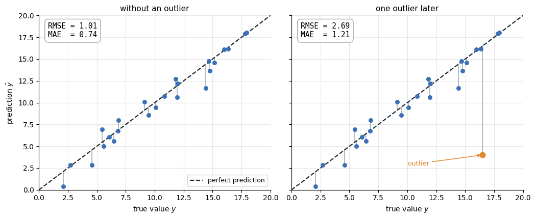 |
| + | |
| + | *The same fit before and after a single outlier: the RMSE nearly triples while the MAE moves far less. Whether that sensitivity is a feature or a flaw depends on how costly large errors are in the application.* |
| + | |
| + | *Remark:* $R^2$ compares the model against the laziest baseline, predicting the mean $\bar{y}$ for every input. $R^2 = 1$ is a perfect fit, $R^2 = 0$ is no better than the baseline, and a negative $R^2$, worse than the baseline, is validation's way of saying the model learned nothing. Unlike the RMSE and MAE it is scale-free, so it compares across targets in different units. |
| + | |
| + | ## 2.7 Classification metrics: beyond a single error rate |
| + | |
| + | For classification, the number the validation reports need not be the raw loss. A trained classifier makes four kinds of calls: true and false positives, true and false negatives. Counting them on held-out data gives the confusion matrix, here for 29 examples: |
| + | |
| + | | | predicted $+$ | predicted $-$ | total | |
| + | | --- | --- | --- | --- | |
| + | | actually $+$ | TP = 11 | FN = 3 | 14 | |
| + | | actually $-$ | FP = 5 | TN = 10 | 15 | |
| + | |
| + | Every headline metric is a ratio of these four cells: |
| + | |
| + | | Metric | Formula | Here | Reads as | |
| + | | --- | --- | --- | --- | |
| + | | Accuracy | $(TP+TN)/\text{total}$ | $21/29 \approx 0.72$ | fraction correct overall | |
| + | | Recall (true positive rate) | $TP/(TP+FN)$ | $11/14 \approx 0.79$ | positives that were found | |
| + | | Precision | $TP/(TP+FP)$ | $11/16 \approx 0.69$ | flagged positives that are right | |
| + | | Specificity | $TN/(TN+FP)$ | $10/15 \approx 0.67$ | negatives that were kept | |
| + | | False positive rate | $FP/(FP+TN)$ | $5/15 \approx 0.33$ | negatives that were flagged | |
| + | | F1 score | $2\,\text{Pr}\cdot\text{Re}/(\text{Pr}+\text{Re})$ | $\approx 0.73$ | precision-recall balance | |
| + | |
| + | *Remark:* accuracy alone can mislead. With 1% positives, always predicting "negative" scores 99% accuracy while finding nothing. Precision and recall keep score where it matters. |
| + | |
| + | A classifier that outputs a score or a probability does not produce one confusion matrix but a family of them: sliding the decision threshold trades false positives against false negatives. |
| + | |
| + | 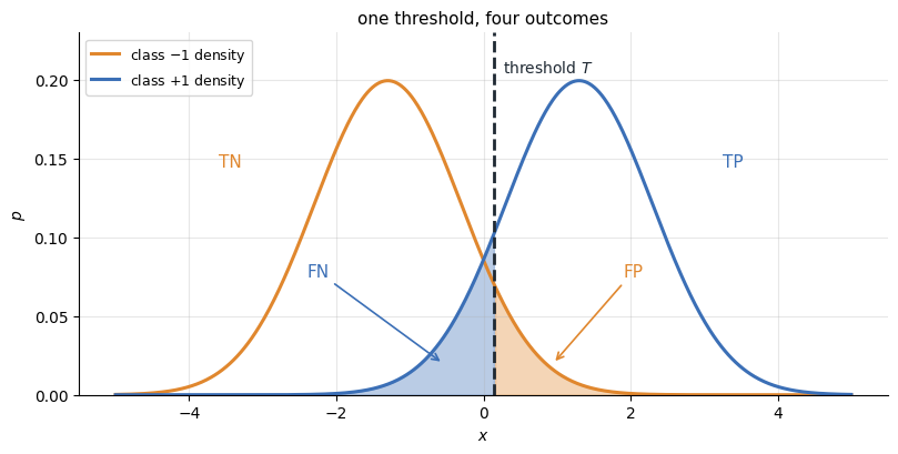 |
| + | |
| + | *Everything right of the threshold is called positive. Pushing the threshold right shrinks the false positives (orange area) but grows the false negatives (blue area), and vice versa.* |
| + | |
| + | Sweeping the threshold and plotting the trade-off gives the ROC curve (recall against false positive rate, perfect is the top-left corner) and the precision-recall curve (perfect is the top-right corner). Two classifiers are compared by their whole curves, or by the area under them, rather than by a single threshold's numbers. |
| + | |
| + | 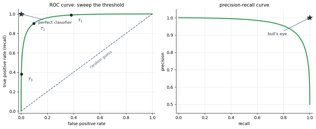 |
| + | |
| + | *Each point on a curve is one threshold: $T_1$ permissive, $T_3$ strict. The closer the curve bends toward its perfect corner, the better the classifier at every trade-off.* |
| + | |
| + | *Remark:* this is what "a metric matched to the problem" means: compute these on the validation folds above to choose a model, and once, on the test set, to report it. |
| + | |
| + | ## 2.8 Common validation pitfalls |
| Honest validation is harder than it looks, and real data often breaks the usual assumptions in three ways. | |
| @@ 140,7 194,7 @@ | |
| *Remark:* the honest question behind every split is the same. Would this have been knowable at the time, from data the model actually had? | |
| - | ## 2.7 The curse of dimensionality |
| + | ## 2.9 The curse of dimensionality |
| Everything above rests on the sample standing in for the population near the points that matter. In high dimension that assumption degrades, and it degrades fast. Suppose the inputs fill the unit hypercube $[0,1]^d$ and we want a neighbourhood around a point that captures a fraction $r$ of the data. A sub-cube containing a fraction $r$ of the volume must have edge length: | |
| /dev/null .. en/Machine Learning/02 General concepts/regression-metrics.png | |
| /dev/null .. en/Machine Learning/02 General concepts/roc-pr-curves.png | |
| /dev/null .. en/Machine Learning/02 General concepts/threshold-metrics.png | |
| en/Machine Learning/03 Probabilistic formulation.md .. | |
| @@ 2,13 2,6 @@ | |
| Probability is the language machine learning uses to handle uncertainty. This module sets out the rules for discrete and continuous variables, takes a first look at information theory, shows the Bayesian way of turning probabilities into decisions, and defines the two estimation principles the course returns to again and again: maximum likelihood and maximum a posteriori. | |
| - | **Objectives** |
| - | - State the rules of probability for discrete and continuous variables. |
| - | - Relate joint, conditional, and marginal probabilities by the sum and product rules and by Bayes' rule. |
| - | - Measure uncertainty with entropy, cross-entropy, and the Kullback-Leibler divergence. |
| - | - Make the decision that minimizes expected loss, and recover the maximum-a-posteriori classifier. |
| - | - Define the maximum-likelihood and maximum-a-posteriori estimators. |
| - | |
| ## 3.1 Probability, discrete and continuous | |
| A random variable takes values with probabilities that are non-negative and sum or integrate to one. A discrete variable has a probability mass function, a continuous one a probability density function: | |
| @@ 59,21 52,21 @@ | |
| ## 3.5 Maximum likelihood and maximum a posteriori | |
| - | We rarely know the true distribution, so we estimate its parameters $\theta$ from data. Maximum likelihood picks the $\theta$ that makes the observed data most probable, usually maximized as a sum of log-likelihoods over the $m$ examples: |
| + | We rarely know the true distribution, so we estimate its parameters $w$ from data. Maximum likelihood picks the $w$ that makes the observed data most probable, usually maximized as a sum of log-likelihoods over the $m$ examples: |
| - | $$\boxed{ \theta_{\mathrm{MLE}} = \arg\max_\theta \sum_{i=1}^{m} \log p(x^{(i)} \mid \theta) }$$ |
| + | $$\boxed{ w_{\mathrm{MLE}} = \arg\max_w \sum_{i=1}^{m} \log p(x^{(i)} \mid w) }$$ |
| - | In supervised learning the model parameterizes the conditional $p(y \mid x; \theta)$, so the same principle applies to the conditional likelihood of the targets: |
| + | In supervised learning the model parameterizes the conditional $p(y \mid x; w)$, so the same principle applies to the conditional likelihood of the targets: |
| - | $$\boxed{ \ell(\theta) = \sum_{i=1}^{m} \log p\!\left(y^{(i)} \mid x^{(i)}; \theta\right) }$$ |
| + | $$\boxed{ \ell(w) = \sum_{i=1}^{m} \log p\!\left(y^{(i)} \mid x^{(i)}; w\right) }$$ |
| - | Maximizing $\ell$ is the same as minimizing the cost $J(\theta) = -\ell(\theta)$, so the likelihood view and the cost-minimization view of [General concepts](/en/Machine%20Learning/02%20General%20concepts) are two faces of one objective. |
| + | Maximizing $\ell$ is the same as minimizing the cost $J(w) = -\ell(w)$, so the likelihood view and the cost-minimization view of [General concepts](/en/Machine%20Learning/02%20General%20concepts) are two faces of one objective. |
| - | Maximum a posteriori instead maximizes the posterior, which multiplies the likelihood by a prior on $\theta$: |
| + | Maximum a posteriori instead maximizes the posterior, which multiplies the likelihood by a prior on $w$: |
| - | $$\boxed{ \theta_{\mathrm{MAP}} = \arg\max_\theta \; p(D \mid \theta)\, p(\theta) }$$ |
| + | $$\boxed{ w_{\mathrm{MAP}} = \arg\max_w \; p(D \mid w)\, p(w) }$$ |
| - | *Remark:* maximum a posteriori is maximum likelihood plus a prior. A Gaussian prior on $\theta$ becomes an L2 penalty and a Laplace prior an L1 penalty, which is exactly the regularization of the next module. With abundant data the prior washes out and the two estimators agree. |
| + | *Remark:* maximum a posteriori is maximum likelihood plus a prior. A Gaussian prior on $w$ becomes an L2 penalty and a Laplace prior an L1 penalty, which is exactly the regularization of the next module. With abundant data the prior washes out and the two estimators agree. |
| *The next module turns these principles into a first concrete model: linear regression, where maximum likelihood and maximum a posteriori both land on closed-form fits.* | |
| en/Machine Learning/04 Linear regression.md .. | |
| @@ 2,21 2,13 @@ | |
| Linear regression predicts a continuous target from a linear score. This module follows one thread from end to end: pose the model, fit it to noisy data by least squares, justify that objective by maximum likelihood, regularize it by maximum a posteriori (ridge, then its selecting cousin the lasso), then widen the model with basis functions and multiple outputs, where the same two closed forms return unchanged. | |
| - | **Objectives** |
| - | - Write the linear model and read its prediction as a line, a plane, or a hyperplane. |
| - | - Pose the fitting problem on noisy data and state the least-squares objective. |
| - | - Show that maximum likelihood under Gaussian noise is exactly least squares, and derive the normal equation. |
| - | - Derive ridge regression (weight decay) from maximum a posteriori, in closed form. |
| - | - Contrast the ridge and lasso penalties: shrinking versus selecting. |
| - | - Generalize the model with basis functions and to multiple outputs, keeping the same closed forms. |
| - | |
| ## 4.1 The linear model | |
| The hypothesis is linear in the augmented input $x \in \mathbb{R}^{n+1}$ with $x_0 = 1$, the convention of the [Introduction](/en/Machine%20Learning/01%20Introduction): | |
| - | $$\boxed{ h_\theta(x) = \theta^T x = \theta_0 + \theta_1 x_1 + \dots + \theta_n x_n }$$ |
| + | $$\boxed{ h_w(x) = w^T x = w_0 + w_1 x_1 + \dots + w_n x_n }$$ |
| - | $\theta_0$ is the bias (the intercept) and the remaining coordinates are the weights, and folding the bias into the dot product is exactly what the $x_0 = 1$ convention buys. Geometrically, the prediction is a line for $n = 1$, a plane for $n = 2$, and a hyperplane beyond. |
| + | $w_0$ is the bias (the intercept) and the remaining coordinates are the weights, and folding the bias into the dot product is exactly what the $x_0 = 1$ convention buys. Geometrically, the prediction is a line for $n = 1$, a plane for $n = 2$, and a hyperplane beyond. |
| 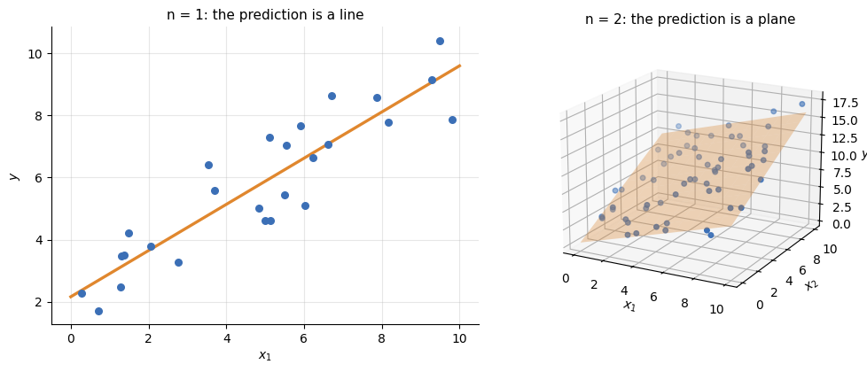 | |
| @@ 24,13 16,13 @@ | |
| ## 4.2 The problem to solve | |
| - | Given the training set $\{(x^{(i)}, y^{(i)})\}_{i=1}^{m}$, ideally we would have $h_\theta(x^{(i)}) = y^{(i)}$ at every point. Real targets are noisy (measurement error, unmodelled factors), so no line passes through them all, and the goal becomes to make the smallest total error. Least squares takes the squared residual as the error and sums it over the training set: |
| + | Given the training set $\{(x^{(i)}, y^{(i)})\}_{i=1}^{m}$, ideally we would have $h_w(x^{(i)}) = y^{(i)}$ at every point. Real targets are noisy (measurement error, unmodelled factors), so no line passes through them all, and the goal becomes to make the smallest total error. Least squares takes the squared residual as the error and sums it over the training set: |
| - | $$\boxed{ \theta^{*} = \arg\min_\theta \; \sum_{i=1}^{m}\left(\theta^T x^{(i)} - y^{(i)}\right)^2 }$$ |
| + | $$\boxed{ w^{*} = \arg\min_w \; \sum_{i=1}^{m}\left(w^T x^{(i)} - y^{(i)}\right)^2 }$$ |
| 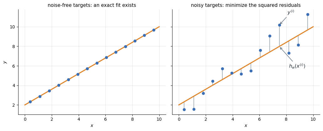 | |
| - | *Left: if the targets were noise-free, the model could pass through every point. Right: real targets scatter around the trend, so each point leaves a residual between $y^{(i)}$ and the prediction $h_\theta(x^{(i)})$, and the fit minimizes their sum of squares (grey segments).* |
| + | *Left: if the targets were noise-free, the model could pass through every point. Right: real targets scatter around the trend, so each point leaves a residual between $y^{(i)}$ and the prediction $h_w(x^{(i)})$, and the fit minimizes their sum of squares (grey segments).* |
| *Remark:* why the square rather than, say, the absolute value? Because this choice is provably optimal when the noise is Gaussian, a classic interview question that the next section unpacks. | |
| @@ 38,77 30,125 @@ | |
| Give the data a generative story, using the estimation principle of [Probabilistic formulation](/en/Machine%20Learning/03%20Probabilistic%20formulation): each target is the linear prediction plus independent Gaussian noise, | |
| - | $$\boxed{ y^{(i)} = \theta^T x^{(i)} + \varepsilon^{(i)}, \quad \varepsilon^{(i)} \sim \mathcal{N}(0, \sigma^2) }$$ |
| + | $$\boxed{ y^{(i)} = w^T x^{(i)} + \varepsilon^{(i)}, \quad \varepsilon^{(i)} \sim \mathcal{N}(0, \sigma^2) }$$ |
| + | |
| + | so $p(y^{(i)} \mid x^{(i)}; w) = \mathcal{N}(w^T x^{(i)}, \sigma^2)$. Maximum likelihood picks the parameters under which the observed targets are the most probable, and it delivers two results. First, maximizing the likelihood is exactly minimizing the sum of squared errors: |
| + | |
| + | $$\boxed{ w_{\mathrm{MLE}} = \arg\max_w \; p(y \mid X; w) = \arg\min_w \; \sum_{i=1}^{m}\left(y^{(i)} - w^T x^{(i)}\right)^2 }$$ |
| + | |
| + | Second, the minimizer has a closed form, the normal equation, with $X$ the design matrix whose rows are the $x^{(i)T}$: |
| + | |
| + | $$\boxed{ w_{\mathrm{MLE}} = (X^T X)^{-1}X^T y }$$ |
| + | |
| + | one matrix solve away from the data. |
| + | |
| + | *Remark:* the first box is the most important fact of the module. Least squares is not a convenient convention, it is the maximum-likelihood estimate under Gaussian noise. |
| - | so $p(y^{(i)} \mid x^{(i)}; \theta) = \mathcal{N}(\theta^T x^{(i)}, \sigma^2)$. The log-likelihood of the $m$ i.i.d. examples separates into a constant and the sum of squares: |
| + | <details class="proof"> |
| + | <summary>Proof: maximizing the likelihood is minimizing the squared error</summary> |
| - | $$\ell(\theta) = \sum_{i=1}^{m} \log \mathcal{N}\!\left(y^{(i)} \mid \theta^T x^{(i)}, \sigma^2\right) = -\frac{m}{2}\log(2\pi\sigma^2) \;-\; \frac{1}{2\sigma^2}\sum_{i=1}^{m}\left(y^{(i)} - \theta^T x^{(i)}\right)^2$$ |
| + | The examples are i.i.d., so the likelihood of the whole training set factorizes into a product of Gaussian densities: |
| - | Neither the constant nor the positive factor $\tfrac{1}{2\sigma^2}$ moves the argmax, so: |
| + | $$p(y \mid X; w) = \prod_{i=1}^{m} p(y^{(i)} \mid x^{(i)}; w) = \prod_{i=1}^{m} \frac{1}{\sqrt{2\pi\sigma^2}}\, \exp\!\left(-\frac{\left(y^{(i)} - w^T x^{(i)}\right)^2}{2\sigma^2}\right)$$ |
| - | $$\boxed{ \arg\max_\theta \; \ell(\theta) = \arg\min_\theta \; \sum_{i=1}^{m}\left(y^{(i)} - \theta^T x^{(i)}\right)^2 }$$ |
| + | The logarithm is increasing, so it preserves the argmax and turns the product into a sum, the log-likelihood, which separates into a constant and the sum of squares: |
| - | *Remark:* this equivalence is the most important fact of the module. Least squares is not a convenient convention, it is the maximum-likelihood estimate under Gaussian noise. |
| + | $$\ell(w) = \sum_{i=1}^{m} \log \mathcal{N}\!\left(y^{(i)} \mid w^T x^{(i)}, \sigma^2\right) = -\frac{m}{2}\log(2\pi\sigma^2) \;-\; \frac{1}{2\sigma^2}\sum_{i=1}^{m}\left(y^{(i)} - w^T x^{(i)}\right)^2$$ |
| - | The maximizer has a closed form. Writing the objective with the design matrix $X$ and setting the gradient to zero, |
| + | The first term does not depend on $w$ and the factor $\tfrac{1}{2\sigma^2}$ is a positive constant, so neither moves the argmax. Maximizing $\ell$ is therefore minimizing the sum of squared errors. $\blacksquare$ |
| - | $$\nabla_\theta\, \lVert X\theta - y \rVert^2 = 2\,X^T(X\theta - y) = 0$$ |
| + | </details> |
| - | $$\boxed{ \theta_{\mathrm{MLE}} = (X^T X)^{-1}X^T y }$$ |
| + | <details class="proof"> |
| + | <summary>Proof: the normal equation</summary> |
| - | the normal equation, one matrix solve away from the data. |
| + | With the design matrix, the sum of squares is the quadratic $\lVert Xw - y \rVert^2$, a convex function of $w$, so its global minimum is the point of zero gradient: |
| + | |
| + | $$\nabla_w\, \lVert Xw - y \rVert^2 = 2\,X^T(Xw - y) = 0 \;\Longleftrightarrow\; X^T X\, w = X^T y$$ |
| + | |
| + | Provided $X^T X$ is invertible (independent features, more examples than features), isolating $w$ gives $w_{\mathrm{MLE}} = (X^T X)^{-1}X^T y$. $\blacksquare$ |
| + | |
| + | </details> |
| ## 4.4 Maximum a posteriori: ridge regression | |
| Maximum likelihood can overfit, especially when the model is flexible. The maximum a posteriori estimate maximizes the posterior instead, which by Bayes' rule is the likelihood times a prior on the parameters, here a zero-mean Gaussian: | |
| - | $$\theta_{\mathrm{MAP}} = \arg\max_\theta \; p(y \mid X, \theta)\, p(\theta), \qquad \theta \sim \mathcal{N}(0, \tau^2 I)$$ |
| + | $$w_{\mathrm{MAP}} = \arg\max_w \; p(y \mid X, w)\, p(w), \qquad w \sim \mathcal{N}(0, \tau^2 I)$$ |
| - | Taking logarithms adds $-\lVert \theta \rVert^2 / 2\tau^2$ to the log-likelihood, and dropping the constants leaves a penalized least squares: |
| + | Two results again. The Gaussian prior turns into an L2 penalty added to least squares: |
| - | $$\boxed{ \theta_{\mathrm{MAP}} = \arg\min_\theta \; \sum_{i=1}^{m}\left(y^{(i)} - \theta^T x^{(i)}\right)^2 + \lambda \lVert \theta \rVert_2^2, \quad \lambda = \frac{\sigma^2}{\tau^2} }$$ |
| + | $$\boxed{ w_{\mathrm{MAP}} = \arg\min_w \; \sum_{i=1}^{m}\left(y^{(i)} - w^T x^{(i)}\right)^2 + \lambda \lVert w \rVert_2^2, \quad \lambda = \frac{\sigma^2}{\tau^2} }$$ |
| - | with, by the same zero-gradient computation, the closed form: |
| + | and the penalized minimizer keeps a closed form: |
| - | $$\boxed{ \theta_{\mathrm{MAP}} = (X^T X + \lambda I)^{-1}X^T y }$$ |
| + | $$\boxed{ w_{\mathrm{MAP}} = (X^T X + \lambda I)^{-1}X^T y }$$ |
| This is ridge regression, and the penalty is often called weight decay. The Gaussian prior became the L2 penalty of [General concepts](/en/Machine%20Learning/02%20General%20concepts), exactly the prior-to-penalty link of [Probabilistic formulation](/en/Machine%20Learning/03%20Probabilistic%20formulation). | |
| - | *Remark:* $\lambda \to 0$ recovers maximum likelihood, and a growing $\lambda$ shrinks $\theta$ toward zero and fights overfitting. A stronger prior (small $\tau$) means a larger $\lambda$. Note also that $X^T X + \lambda I$ is always invertible for $\lambda > 0$, which rescues least squares exactly where it breaks down: strongly correlated features, or more features than examples. |
| + | *Remark:* $\lambda \to 0$ recovers maximum likelihood, and a growing $\lambda$ shrinks $w$ toward zero and fights overfitting. A stronger prior (small $\tau$) means a larger $\lambda$. Note also that $X^T X + \lambda I$ is always invertible for $\lambda > 0$, which rescues least squares exactly where it breaks down: strongly correlated features, or more features than examples. |
| - | ## 4.5 The lasso: a penalty that selects |
| + | <details class="proof"> |
| + | <summary>Proof: the Gaussian prior becomes the L2 penalty</summary> |
| - | The ridge penalty came from a Gaussian prior. A Laplace prior yields the L1 penalty instead, the link noted in [Probabilistic formulation](/en/Machine%20Learning/03%20Probabilistic%20formulation): |
| + | By Bayes' rule the posterior is |
| + | |
| + | $$p(w \mid y, X) = \frac{p(y \mid X, w)\, p(w)}{p(y \mid X)}$$ |
| - | $$\boxed{ \theta_{\mathrm{lasso}} = \arg\min_\theta \; \sum_{i=1}^{m}\left(y^{(i)} - \theta^T x^{(i)}\right)^2 + \lambda \lVert \theta \rVert_1 }$$ |
| + | and the denominator does not depend on $w$, so maximizing the posterior is maximizing the likelihood times the prior. The prior covariance is generally unknown, so it is assumed isotropic, $\tau^2 I$, which gives the density |
| - | The change looks small and its consequence is large: the lasso drives some coefficients to exactly zero, so it selects variables while it fits. Unlike ridge it has no closed form (the penalty is not differentiable at zero), so it is fitted by convex solvers. The reason for the selection is geometric. The constraint region $\lVert \theta \rVert_1 \le t$ is a diamond with corners on the axes, and the elliptical contours of the squared error tend to touch it first at a corner, where a coordinate is zero. The rounded L2 ball has no corners, so ridge shrinks every coefficient smoothly but never zeroes one: ridge stabilizes, the lasso selects. |
| + | $$p(w) = \frac{1}{(2\pi\tau^2)^{(n+1)/2}}\, \exp\!\left(-\frac{\lVert w \rVert^2}{2\tau^2}\right)$$ |
| - |  |
| + | Taking logarithms and reusing the log-likelihood $\ell(w)$ from the previous proof, |
| - | *The rounded L2 ball is touched off the axes, keeping every coefficient nonzero, while the L1 diamond is touched at a corner, setting a coefficient to exactly zero.* |
| + | $$\log p(y \mid X, w) + \log p(w) = \mathrm{const} \;-\; \frac{1}{2\sigma^2}\sum_{i=1}^{m}\left(y^{(i)} - w^T x^{(i)}\right)^2 \;-\; \frac{1}{2\tau^2}\lVert w \rVert^2$$ |
| - | As $\lambda$ grows, more coefficients cross to zero, tracing the regularization path from the full model down to the empty one. |
| + | where the constant gathers every term independent of $w$. Multiplying by $-2\sigma^2$, a negative constant that flips the argmax into an argmin, leaves |
| + | |
| + | $$w_{\mathrm{MAP}} = \arg\min_w \; \sum_{i=1}^{m}\left(y^{(i)} - w^T x^{(i)}\right)^2 + \frac{\sigma^2}{\tau^2}\, \lVert w \rVert^2$$ |
| + | |
| + | and $\lambda = \sigma^2 / \tau^2$ names the ratio: the noisier the data or the tighter the prior, the heavier the penalty. $\blacksquare$ |
| + | |
| + | </details> |
| + | |
| + | <details class="proof"> |
| + | <summary>Proof: the ridge closed form</summary> |
| + | |
| + | In matrix form the objective is $\lVert Xw - y \rVert^2 + \lambda \lVert w \rVert^2$, still a convex quadratic, so the zero-gradient condition finds its global minimum: |
| + | |
| + | $$\nabla_w \left( \lVert Xw - y \rVert^2 + \lambda \lVert w \rVert^2 \right) = 2\,X^T(Xw - y) + 2\lambda w = 0 \;\Longleftrightarrow\; (X^T X + \lambda I)\, w = X^T y$$ |
| + | |
| + | For $\lambda > 0$ the matrix $X^T X + \lambda I$ is positive definite, hence invertible, with no condition on $X$ this time: for any $v \neq 0$, $v^T (X^T X + \lambda I)\, v = \lVert X v \rVert^2 + \lambda \lVert v \rVert^2 > 0$. Isolating $w$ gives $w_{\mathrm{MAP}} = (X^T X + \lambda I)^{-1} X^T y$. $\blacksquare$ |
| + | |
| + | </details> |
| + | |
| + | ## 4.5 The lasso: a penalty that selects |
| + | |
| + | The ridge penalty came from a Gaussian prior. A Laplace prior yields the L1 penalty instead, the link noted in [Probabilistic formulation](/en/Machine%20Learning/03%20Probabilistic%20formulation): |
| - |  |
| + | $$\boxed{ w_{\mathrm{lasso}} = \arg\min_w \; \sum_{i=1}^{m}\left(y^{(i)} - w^T x^{(i)}\right)^2 + \lambda \lVert w \rVert_1 }$$ |
| - | *Each coefficient shrinks as $\lambda$ increases and then hits exactly zero, so the lasso yields a compact, interpretable subset of regressors.* |
| + | The change looks small, its consequences are not: |
| - | *Remark:* the elastic net blends the two penalties, $\lambda\left(\alpha \lVert \theta \rVert_1 + (1-\alpha)\lVert \theta \rVert_2^2\right)$, keeping the lasso's selection with the ridge's stability under correlated features. As always, $\lambda$ is chosen by the cross-validation of [General concepts](/en/Machine%20Learning/02%20General%20concepts), often taking the largest $\lambda$ within one standard error of the best for a simpler model. |
| + | - **It selects.** The lasso drives some coefficients to exactly zero, performing variable selection while it fits. Ridge only shrinks and never zeroes: ridge stabilizes, the lasso selects. |
| + | - **The reason is geometric.** The constraint region $\lVert w \rVert_1 \le t$ is a diamond with corners on the axes, and the elliptical contours of the squared error tend to touch a corner first, where a coordinate is zero. The rounded L2 ball has no corners to catch. |
| + | - **$\lambda$ traces a path.** As $\lambda$ grows, coefficients hit exactly zero one after another, from the full model down to the empty one. As always, $\lambda$ is chosen by the cross-validation of [General concepts](/en/Machine%20Learning/02%20General%20concepts), often the largest $\lambda$ within one standard error of the best. |
| + | - **No closed form.** The L1 penalty is not differentiable at zero, so the lasso is fitted by convex solvers rather than a formula. |
| + | - **The elastic net** blends the two penalties, $\lambda\left(\alpha \lVert w \rVert_1 + (1-\alpha)\lVert w \rVert_2^2\right)$, keeping the lasso's selection with the ridge's stability under correlated features. |
| *Remark:* prediction is not inference. Selecting variables with the lasso and then reporting textbook standard errors on the same data is invalid, the winner's curse again: the intervals ignore that the data already chose the variables. Honest inference needs sample splitting or a debiased estimator, the doorway to causal machine learning. | |
| - | ## 4.6 Basis functions: nonlinear in $x$, linear in $\theta$ |
| + | ## 4.6 Basis functions: nonlinear in $x$, linear in $w$ |
| A straight line is often too rigid: the underfitting of [General concepts](/en/Machine%20Learning/02%20General%20concepts) appeared precisely when a low-capacity model met a curved trend. The fix is not to abandon the linear machinery but to project the input into a larger space, where the relationship is linear: | |
| - | $$\boxed{ h_\theta(x) = \theta^T \phi(x) = \sum_{j=0}^{M-1} \theta_j\, \phi_j(x), \qquad \phi_0(x) = 1 }$$ |
| + | $$\boxed{ h_w(x) = w^T \phi(x) = \sum_{j=0}^{M-1} w_j\, \phi_j(x), \qquad \phi_0(x) = 1 }$$ |
| - | The $\phi_j$ are basis functions, fixed before training. With $\phi(x) = (1, x, x^2, \dots, x^d)$ they give polynomial regression, the running example of [General concepts](/en/Machine%20Learning/02%20General%20concepts), and the identity $\phi(x) = x$ recovers everything above. The model can now be wildly nonlinear in $x$ yet stays linear in $\theta$, so nothing changes in the fit: stack the $\phi(x^{(i)})^T$ as the rows of the design matrix $\Phi \in \mathbb{R}^{m \times M}$ and the two closed forms return verbatim: |
| + | The $\phi_j$ are basis functions, fixed before training. With $\phi(x) = (1, x, x^2, \dots, x^d)$ they give polynomial regression, the running example of [General concepts](/en/Machine%20Learning/02%20General%20concepts), and the identity $\phi(x) = x$ recovers everything above. The model can now be wildly nonlinear in $x$ yet stays linear in $w$, so nothing changes in the fit: stack the $\phi(x^{(i)})^T$ as the rows of the design matrix $\Phi \in \mathbb{R}^{m \times M}$ and the two closed forms return verbatim: |
| - | $$\boxed{ \theta_{\mathrm{MLE}} = (\Phi^T \Phi)^{-1}\Phi^T y, \qquad \theta_{\mathrm{MAP}} = (\Phi^T \Phi + \lambda I)^{-1}\Phi^T y }$$ |
| + | $$\boxed{ w_{\mathrm{MLE}} = (\Phi^T \Phi)^{-1}\Phi^T y, \qquad w_{\mathrm{MAP}} = (\Phi^T \Phi + \lambda I)^{-1}\Phi^T y }$$ |
| - | *Remark:* the basis (its family and its size $M$) is a hyperparameter, chosen before training, while $\theta$ is learned. Choosing $M$ and $\lambda$ is the model-selection problem settled by the cross-validation of [General concepts](/en/Machine%20Learning/02%20General%20concepts). |
| + | *Remark:* the basis (its family and its size $M$) is a hyperparameter, chosen before training, while $w$ is learned. Choosing $M$ and $\lambda$ is the model-selection problem settled by the cross-validation of [General concepts](/en/Machine%20Learning/02%20General%20concepts). |
| ## 4.7 Multiple outputs | |
| @@ 126,10 166,10 @@ | |
| | | Formula | | |
| | --- | --- | | |
| - | | Model | $h_\theta(x) = \theta^T \phi(x)$ | |
| - | | Maximum likelihood (least squares) | $\theta_{\mathrm{MLE}} = (\Phi^T \Phi)^{-1}\Phi^T y$ | |
| - | | Maximum a posteriori (ridge) | $\theta_{\mathrm{MAP}} = (\Phi^T \Phi + \lambda I)^{-1}\Phi^T y$ | |
| - | | Parameters, learned | $\theta$ (or $W$ for $K$ outputs) | |
| + | | Model | $h_w(x) = w^T \phi(x)$ | |
| + | | Maximum likelihood (least squares) | $w_{\mathrm{MLE}} = (\Phi^T \Phi)^{-1}\Phi^T y$ | |
| + | | Maximum a posteriori (ridge) | $w_{\mathrm{MAP}} = (\Phi^T \Phi + \lambda I)^{-1}\Phi^T y$ | |
| + | | Parameters, learned | $w$ (or $W$ for $K$ outputs) | |
| | Hyperparameters, chosen by validation | the basis $\phi$ and its size $M$, the penalty $\lambda$ | | |
| *The same linear score, passed through a squashing function instead of read directly, turns regression into classification, the subject of the next module.* | |
| en/Machine Learning/04 Linear regression/ideal-vs-noisy.png .. | |
| en/Machine Learning/04 Linear regression/l1-l2-geometry.png .. /dev/null | |
| en/Machine Learning/04 Linear regression/regularization-path.png .. /dev/null | |
| en/Machine Learning/05 Linear classification.md .. | |
| @@ 1,43 1,26 @@ | |
| # 5. Linear classification | |
| - | Classification predicts a discrete label from the same linear score $\theta^T x$. This module surveys the classical linear classifiers as one menu: least squares, which assumes Gaussian-shaped classes and admits a closed form, and the perceptron and logistic regression, which assume nothing about the distribution and are fitted by gradient descent. Regularization closes the module. |
| - | |
| - | **Objectives** |
| - | - Read a linear classifier as a separating hyperplane whose score tells the side, making prediction one dot product. |
| - | - Situate the classical methods by their assumption (Gaussian or none) and their fit (closed form or gradient descent). |
| - | - Classify by least squares, binary and multiclass, and see where it breaks. |
| - | - Train the perceptron from its criterion, and know its convergence guarantee and its limits. |
| - | - Distinguish batch from stochastic gradient descent, and know that fancier optimizers exist. |
| - | - Fit logistic regression by gradient descent on the cross-entropy, binary and multiclass. |
| - | - Regularize any of these fits with a penalty, the maximum a posteriori view. |
| + | Classification predicts a discrete label from the same linear score $w^T x$. This module surveys the classical linear classifiers as one menu: least squares, which assumes Gaussian-shaped classes and admits a closed form, and the perceptron and logistic regression, which assume nothing about the distribution and are fitted by gradient descent. Regularization closes the module. |
| ## 5.1 The linear separator | |
| A linear classifier assigns the class from the sign of the linear score, and the set of inputs scoring zero is the decision boundary: | |
| - | $$\boxed{ h_\theta(x) = \mathrm{sign}(\theta^T x), \qquad \theta^T x = 0 \ \text{is the boundary} }$$ |
| - | |
| - | The boundary is a hyperplane: a line with two features, a plane with three. The sign of the score says on which side of the hyperplane the input falls, and its magnitude how far from the boundary it sits. With $\theta = (-4, 1, 2)$ (bias first, on the augmented input), the point $x = (3, 2)$ scores $-4 + 3 + 4 = 3$ and falls in front of the hyperplane, while $x = (1, 1)$ scores $-4 + 1 + 2 = -1$ and falls behind it. |
| - | |
| - | *Remark:* two practical advantages follow. Once training is done the training set can be thrown away, and predicting costs a single dot product. |
| + | $$\boxed{ h_w(x) = \mathrm{sign}(w^T x), \qquad w^T x = 0 \ \text{is the boundary} }$$ |
| - | ## 5.2 A menu of methods |
| + | The boundary is a hyperplane: a line with two features, a plane with three. The sign of the score says on which side of the hyperplane the input falls, and its magnitude how far from the boundary it sits. With $w = (-4, 1, 2)$ (bias first, on the augmented input), the point $x = (3, 2)$ scores $-4 + 3 + 4 = 3$ and falls in front of the hyperplane, while $x = (1, 1)$ scores $-4 + 1 + 2 = -1$ and falls behind it. |
| - | The classical methods fit that hyperplane, and they split cleanly by what they assume about the data and how they are solved. |
| + | 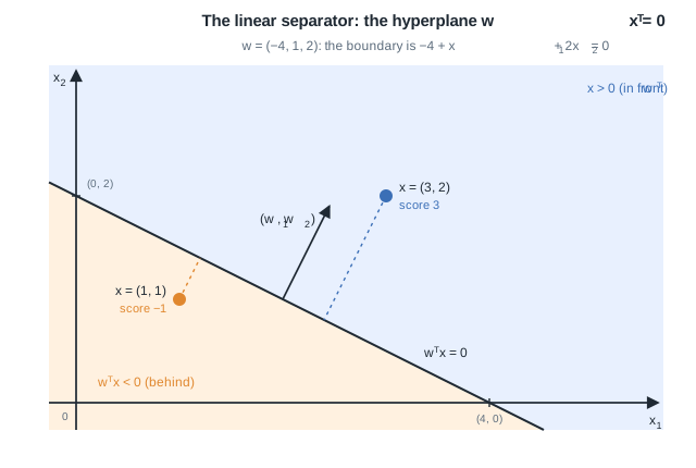 |
| - | | Method | Assumption on the data | How it is fitted | |
| - | | --- | --- | --- | |
| - | | Least squares | Gaussian-shaped classes | closed form (matrix inversion) | |
| - | | Perceptron | none | gradient descent | |
| - | | Logistic regression | none | gradient descent | |
| + | *The hyperplane $w^T x = 0$ splits the input space in two: with $w = (-4, 1, 2)$ the boundary is the line $-4 + x_1 + 2x_2 = 0$, normal to $(w_1, w_2)$. The point $(3, 2)$ scores $3$ and falls in front, $(1, 1)$ scores $-1$ and falls behind, and the magnitude of the score grows with the distance to the boundary (dotted).* |
| - | Least squares inherits the closed-form comfort of [Linear regression](/en/Machine%20Learning/04%20Linear%20regression) and pays for it with a distributional assumption. The other two assume nothing and pay with iterative optimization. |
| + | *Remark:* two practical advantages follow. Once training is done the training set can be thrown away, and predicting costs a single dot product. |
| - | ## 5.3 Least squares as a classifier |
| + | ## 5.2 Least squares as a classifier |
| Code the two classes as $y \in \{-1, +1\}$, treat them as regression targets, and everything from [Linear regression](/en/Machine%20Learning/04%20Linear%20regression) applies verbatim, closed form included: | |
| - | $$\boxed{ \theta = (X^T X)^{-1}X^T y, \qquad h_\theta(x) = \mathrm{sign}(\theta^T x) }$$ |
| + | $$\boxed{ w = (X^T X)^{-1}X^T y, \qquad h_w(x) = \mathrm{sign}(w^T x) }$$ |
| For $K > 2$ classes, code each label as a one-hot row of $Y \in \mathbb{R}^{m \times K}$ and reuse the multiple-output regression of [Linear regression](/en/Machine%20Learning/04%20Linear%20regression), predicting the class with the highest score: | |
| @@ 49,25 32,31 @@ | |
| *Without outliers least squares and logistic regression agree. Adding distant, correctly classified points tilts the least-squares boundary into errors, while logistic regression barely moves.* | |
| - | ## 5.4 The perceptron |
| + | ## 5.3 The perceptron |
| - | ### 5.4.1 Model, loss, and update |
| + | ### 5.3.1 The model: one neuron |
| The first assumption-free method takes the definition of a linear classifier at face value, a dot product followed by a hard activation, the historical neuron: | |
| - | $$\boxed{ h_\theta(x) = \mathrm{sign}(\theta^T x), \qquad y \in \{-1, +1\} }$$ |
| + | $$\boxed{ h_w(x) = \mathrm{sign}(w^T x), \qquad y \in \{-1, +1\} }$$ |
| 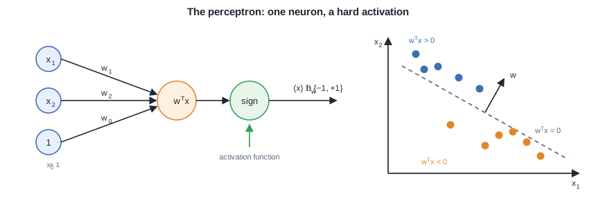 | |
| - | *Left: the perceptron is a single neuron, the weighted inputs summed into the score $\theta^T x$ and passed through a hard sign activation. Right: that sign splits the input space along the hyperplane $\theta^T x = 0$.* |
| + | *Left: the perceptron is a single neuron, the weighted inputs summed into the score $w^T x$ and passed through a hard sign activation. Right: that sign splits the input space along the hyperplane $w^T x = 0$.* |
| - | Fitting needs a loss, and counting mistakes does not work: the count is piecewise constant, so its gradient is zero almost everywhere. The perceptron criterion instead penalizes each misclassified point by how far it sits on the wrong side. A mistake means $y^{(i)}\,\theta^T x^{(i)} < 0$, so over the set $\mathcal{M}$ of misclassified points: |
| + | ### 5.3.2 The loss function: the perceptron criterion |
| - | $$\boxed{ E(\theta) = -\sum_{i \in \mathcal{M}} y^{(i)}\, \theta^T x^{(i)} }$$ |
| + | Fitting needs a loss, and counting mistakes does not work: the count is piecewise constant, so its gradient is zero almost everywhere. The perceptron criterion instead penalizes each misclassified point by how far it sits on the wrong side. A mistake means $y^{(i)}\,w^T x^{(i)} < 0$, so over the set $\mathcal{M}$ of misclassified points: |
| - | always positive and piecewise linear. Minimizing it introduces the workhorse of everything in this course that lacks a closed form, gradient descent: repeatedly step the parameters against the gradient of the loss, scaled by a learning rate $\alpha > 0$: |
| + | $$\boxed{ E(w) = -\sum_{i \in \mathcal{M}} y^{(i)}\, w^T x^{(i)} }$$ |
| - | $$\boxed{\,\theta \leftarrow \theta - \alpha\,\nabla_\theta E(\theta)\,}$$ |
| + | always positive and piecewise linear. |
| + | |
| + | ### 5.3.3 Optimization: gradient descent |
| + | |
| + | Minimizing the criterion introduces the workhorse of everything in this course that lacks a closed form, gradient descent: repeatedly step the parameters against the gradient of the loss, scaled by a learning rate $\alpha > 0$: |
| + | |
| + | $$\boxed{\,w \leftarrow w - \alpha\,\nabla_w E(w)\,}$$ |
| The batch variant computes the gradient over the whole training set before each step, a smooth descent that reads every example every time. The stochastic variant (SGD) steps on one example at a time, cheap and noisy, and is the default on large datasets. If $\alpha$ is too large the iterates can diverge, if too small convergence crawls. | |
| @@ 75,21 64,21 @@ | |
| On a single misclassified example the gradient of the criterion is $-y^{(i)} x^{(i)}$, so the stochastic step is the perceptron update: on a mistake, | |
| - | $$\boxed{ \theta \leftarrow \theta + \alpha\, y^{(i)} x^{(i)} }$$ |
| + | $$\boxed{ w \leftarrow w + \alpha\, y^{(i)} x^{(i)} }$$ |
| - | and no update otherwise. In the $\{0, 1\}$ coding this is the residual-times-input update $\theta_j \leftarrow \theta_j + \alpha\,(y^{(i)} - h_\theta(x^{(i)}))\,x_j^{(i)}$. |
| + | and no update otherwise. In the $\{0, 1\}$ coding this is the residual-times-input update $w_j \leftarrow w_j + \alpha\,(y^{(i)} - h_w(x^{(i)}))\,x_j^{(i)}$. |
| 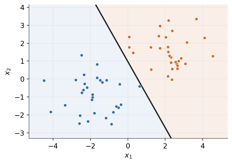 | |
| *The perceptron finds one separating hyperplane, not necessarily the maximum-margin one the support vector machine will choose.* | |
| - | ### 5.4.2 Multiclass perceptron |
| + | ### 5.3.4 Multiclass perceptron |
| - | With $k$ classes, keep one weight vector $\theta_c$ per class and predict the highest-scoring one. On a mistake, reward the true class and penalize the predicted one: |
| + | With $k$ classes, keep one weight vector $w_c$ per class and predict the highest-scoring one. On a mistake, reward the true class and penalize the predicted one: |
| - | $$\boxed{ \hat{y} = \arg\max_c \theta_c^T x, \qquad \theta_{y} \mathrel{+}= \alpha x, \quad \theta_{\hat{y}} \mathrel{-}= \alpha x }$$ |
| + | $$\boxed{ \hat{y} = \arg\max_c w_c^T x, \qquad w_{y} \mathrel{+}= \alpha x, \quad w_{\hat{y}} \mathrel{-}= \alpha x }$$ |
| - | The network view extends naturally: one score neuron per class, and an argmax where the binary perceptron had a sign. Gathering the $\theta_c$ as the columns of a matrix $W \in \mathbb{R}^{(n+1) \times k}$, one product $W^T x$ computes every score at once, and the scores carve the input space into $k$ regions, each claimed by the class whose score is largest. |
| + | The network view extends naturally: one score neuron per class, and an argmax where the binary perceptron had a sign. Gathering the $w_c$ as the columns of a matrix $W \in \mathbb{R}^{(n+1) \times k}$, one product $W^T x$ computes every score at once, and the scores carve the input space into $k$ regions, each claimed by the class whose score is largest. |
| 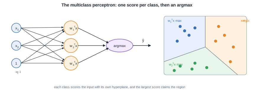 | |
| @@ 99,87 88,165 @@ | |
| $$ W^T x = \begin{bmatrix} -2 & -4 & 1 \\ -4 & 2 & 4 \\ -6 & 4 & -5 \end{bmatrix}\begin{bmatrix} 1 \\ 1.1 \\ -2.0 \end{bmatrix} = \begin{bmatrix} -8.4 \\ -9.8 \\ 8.4 \end{bmatrix} $$ | |
| - | The third score wins, so the input is assigned to class 3. Reading off the third row, that score is $\theta_3^T x = -6 + 4 \times 1.1 + (-5) \times (-2.0) = 8.4$. |
| + | The third score wins, so the input is assigned to class 3. Reading off the third row, that score is $w_3^T x = -6 + 4 \times 1.1 + (-5) \times (-2.0) = 8.4$. |
| - | ### 5.4.3 Convergence and limits |
| + | ### 5.3.5 Convergence and limits |
| If the data is linearly separable the perceptron converges in a finite number of updates, otherwise the weights oscillate forever. And since the criterion is zero on every separating hyperplane, all of them count as "optimal", including those that graze the data. | |
| *Remark:* three upgrades fix these limits, and each one opens a module. A smooth activation and loss give logistic regression, next section. Margins and basis functions lead to the [Support Vector Machine](/en/Machine%20Learning/07%20Support%20Vector%20Machines). Stacking neurons into layers gives [multilayer neural networks](/en/Machine%20Learning/06%20Multilayer%20neural%20networks), the starting point of the Deep Learning course. | |
| - | ## 5.5 Logistic regression |
| + | ## 5.4 Logistic regression |
| - | ### 5.5.1 A smooth activation |
| + | ### 5.4.1 The model: a smooth activation |
| - | Logistic regression keeps the neuron but replaces the hard step with the smooth sigmoid, so the output is the probability of the positive class ($y \in \{0, 1\}$): |
| + | Logistic regression keeps the neuron but replaces the hard step with the smooth sigmoid, so the output is the probability of the positive class ($y \in \{0, 1\}$). It is still written $\hat{y}$, but the estimate of the label is now soft: the perceptron's $\hat{y}$ was a hard class, logistic regression's is a probability, and thresholding it at $\tfrac{1}{2}$ turns it back into a class whenever one is needed: |
| - | $$\boxed{ \phi = p(y = 1 \mid x; \theta) = \sigma(\theta^T x) = \frac{1}{1 + e^{-\theta^T x}} }$$ |
| + | $$\boxed{ \hat{y} = p(y = 1 \mid x; w) = \sigma(w^T x) = \frac{1}{1 + e^{-w^T x}} }$$ |
| 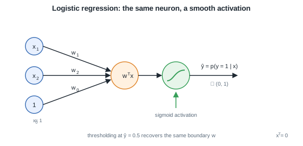 | |
| - | *The same neuron with the step swapped for the sigmoid: the output becomes the probability $\phi = p(y = 1 \mid x)$, and thresholding it at $\tfrac{1}{2}$ recovers the same boundary $\theta^T x = 0$.* |
| + | *The same neuron with the step swapped for the sigmoid: the output becomes the probability $\hat{y} = p(y = 1 \mid x)$, and thresholding it at $\tfrac{1}{2}$ recovers the same boundary $w^T x = 0$.* |
| *Remark:* the sigmoid is not an arbitrary squashing choice. Writing the posterior with Bayes' rule gives $p(C_1 \mid x) = 1/(1 + e^{-a})$ with $a = \ln \frac{p(x \mid C_1)\,p(C_1)}{p(x \mid C_0)\,p(C_0)}$, so a well-trained logistic output is exactly a posterior probability. | |
| - | ### 5.5.2 Cross-entropy and its gradient |
| + | ### 5.4.2 The loss function: cross-entropy |
| The likelihood of Bernoulli labels, taken through $-\log$, gives the cross-entropy loss: | |
| - | $$\boxed{ L(\theta) = -\sum_{i=1}^{m}\left[ y^{(i)}\log \phi^{(i)} + (1 - y^{(i)})\log(1 - \phi^{(i)}) \right] }$$ |
| + | $$\boxed{ L(w) = -\sum_{i=1}^{m}\left[ y^{(i)}\log \hat{y}^{(i)} + (1 - y^{(i)})\log(1 - \hat{y}^{(i)}) \right] }$$ |
| + | |
| + | <details class="proof"> |
| + | <summary>Proof: maximum likelihood gives the cross-entropy</summary> |
| + | |
| + | The model says each label is a Bernoulli draw with success probability $\hat{y}^{(i)} = \sigma(w^T x^{(i)})$, and both cases fold into one expression: |
| + | |
| + | $$p(y^{(i)} \mid x^{(i)}; w) = \left(\hat{y}^{(i)}\right)^{y^{(i)}}\left(1 - \hat{y}^{(i)}\right)^{1 - y^{(i)}}$$ |
| + | |
| + | since $y^{(i)} \in \{0, 1\}$ selects the factor: the expression is $\hat{y}^{(i)}$ when $y^{(i)} = 1$ and $1 - \hat{y}^{(i)}$ when $y^{(i)} = 0$. The examples are i.i.d., so the likelihood of the training set factorizes, as it did in [Linear regression](/en/Machine%20Learning/04%20Linear%20regression): |
| + | |
| + | $$p(y \mid X; w) = \prod_{i=1}^{m} \left(\hat{y}^{(i)}\right)^{y^{(i)}}\left(1 - \hat{y}^{(i)}\right)^{1 - y^{(i)}}$$ |
| + | |
| + | The logarithm preserves the argmax, turns the product into a sum and brings the exponents down: |
| + | |
| + | $$\ell(w) = \sum_{i=1}^{m}\left[ y^{(i)}\log \hat{y}^{(i)} + (1 - y^{(i)})\log(1 - \hat{y}^{(i)}) \right]$$ |
| + | |
| + | Maximizing $\ell$ is minimizing $-\ell$, which is exactly $L(w)$. The cross-entropy is the negative Bernoulli log-likelihood, the same estimation principle that made least squares the answer under Gaussian noise. $\blacksquare$ |
| + | |
| + | </details> |
| + | |
| + | ### 5.4.3 Optimization: gradient descent |
| Unlike least squares, this loss has no closed-form minimizer: the sigmoid makes the stationarity equations transcendental, so the fit falls to the same gradient descent as the perceptron. Differentiating the cross-entropy through the sigmoid rewards the effort: almost everything cancels and the gradient collapses to the residual times the input: | |
| - | $$\boxed{ \theta_j \leftarrow \theta_j - \alpha \sum_{i=1}^{m}\left(\phi^{(i)} - y^{(i)}\right)x_j^{(i)} }$$ |
| + | $$\boxed{ w_j \leftarrow w_j - \alpha \sum_{i=1}^{m}\left(\hat{y}^{(i)} - y^{(i)}\right)x_j^{(i)} }$$ |
| + | |
| + | <details class="proof"> |
| + | <summary>Proof: the gradient collapses to the residual times the input</summary> |
| + | |
| + | Write the score $z^{(i)} = w^T x^{(i)}$, so that $\hat{y}^{(i)} = \sigma(z^{(i)})$. The derivation rests on one identity, the sigmoid differentiating into itself: |
| - | *Remark:* unlike the perceptron, the gradient involves every training point, not only the misclassified ones: each point pulls in proportion to its residual $\phi^{(i)} - y^{(i)}$. That is what makes logistic regression more stable than the perceptron and usable on non-separable data. |
| + | $$\sigma'(z) = \frac{e^{-z}}{\left(1 + e^{-z}\right)^2} = \frac{1}{1 + e^{-z}} \cdot \frac{e^{-z}}{1 + e^{-z}} = \sigma(z)\left(1 - \sigma(z)\right)$$ |
| + | |
| + | since $\tfrac{e^{-z}}{1 + e^{-z}} = 1 - \sigma(z)$. Now take the loss of a single example, $L^{(i)} = -\left[y^{(i)}\log \hat{y}^{(i)} + (1 - y^{(i)})\log(1 - \hat{y}^{(i)})\right]$, and follow the chain rule through its three stages, loss to output, output to score, score to weight: |
| + | |
| + | $$\frac{\partial L^{(i)}}{\partial \hat{y}^{(i)}} = -\frac{y^{(i)}}{\hat{y}^{(i)}} + \frac{1 - y^{(i)}}{1 - \hat{y}^{(i)}} = \frac{\hat{y}^{(i)} - y^{(i)}}{\hat{y}^{(i)}\left(1 - \hat{y}^{(i)}\right)}, \qquad \frac{\partial \hat{y}^{(i)}}{\partial z^{(i)}} = \hat{y}^{(i)}\left(1 - \hat{y}^{(i)}\right), \qquad \frac{\partial z^{(i)}}{\partial w_j} = x_j^{(i)}$$ |
| + | |
| + | (the first equality puts the two fractions over the common denominator $\hat{y}^{(i)}(1 - \hat{y}^{(i)})$, and the second is the sigmoid identity above). Multiplying the three, the denominator of the first factor is exactly the second factor, and everything cancels: |
| + | |
| + | $$\frac{\partial L^{(i)}}{\partial w_j} = \frac{\hat{y}^{(i)} - y^{(i)}}{\hat{y}^{(i)}\left(1 - \hat{y}^{(i)}\right)} \cdot \hat{y}^{(i)}\left(1 - \hat{y}^{(i)}\right) \cdot x_j^{(i)} = \left(\hat{y}^{(i)} - y^{(i)}\right) x_j^{(i)}$$ |
| + | |
| + | Summing over the training set gives $\partial L / \partial w_j = \sum_{i=1}^{m} (\hat{y}^{(i)} - y^{(i)})\, x_j^{(i)}$, and plugging this gradient into the descent rule $w \leftarrow w - \alpha\, \nabla_w L$ is the boxed update. $\blacksquare$ |
| + | |
| + | </details> |
| + | |
| + | *Remark:* unlike the perceptron, the gradient involves every training point, not only the misclassified ones: each point pulls in proportion to its residual $\hat{y}^{(i)} - y^{(i)}$. That is what makes logistic regression more stable than the perceptron and usable on non-separable data. |
| 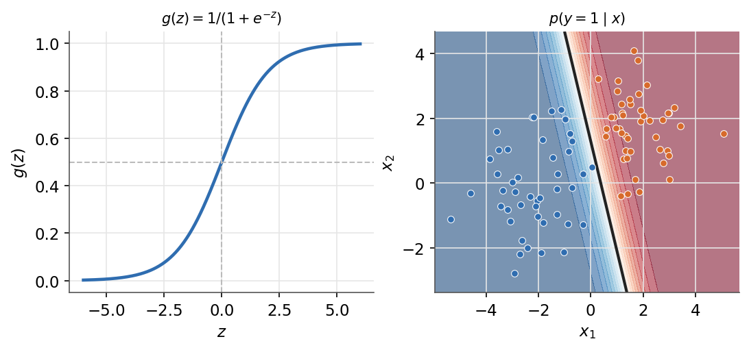 | |
| *Left: the sigmoid maps any score into the interval (0, 1). Right: the decision boundary and the predicted probability.* | |
| - | ### 5.5.3 Multiclass: the softmax |
| + | ### 5.4.4 Multiclass: the softmax |
| + | |
| + | For $k$ classes the sigmoid generalizes to the softmax: one weight vector $w_c$, hence one score, per class, exponentials that make the scores positive, and a normalization that turns them into a distribution. Writing $\hat{y}_c$ for the predicted probability of class $c$, as $\hat{y}$ was the probability of the positive class above: |
| + | |
| + | $$\boxed{ \hat{y}_c = p(y = c \mid x; w) = \frac{\exp(w_c^T x)}{\sum_{j=1}^{k}\exp(w_j^T x)} }$$ |
| - | For $k$ classes the sigmoid generalizes to the softmax, one weight vector per class, normalized into a distribution: |
| + | 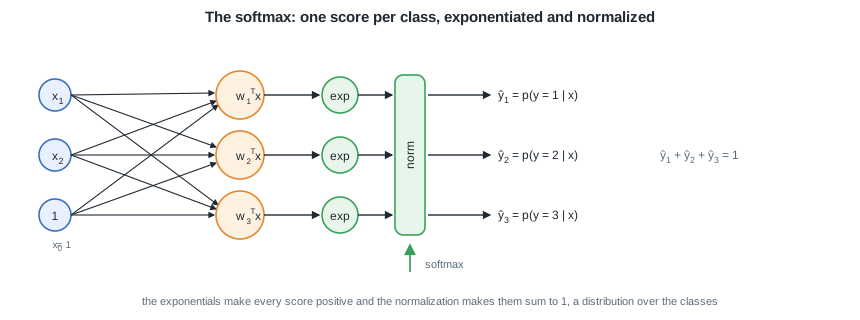 |
| - | $$\boxed{ p(y = c \mid x; \theta) = \frac{\exp(\theta_c^T x)}{\sum_{j=1}^{k}\exp(\theta_j^T x)} }$$ |
| + | *The multiclass network with a softmax head: each class scores the input, the exponentials make the scores positive, and the normalization turns them into probabilities that sum to 1. It is the multiclass perceptron's network with the argmax replaced by a smooth, differentiable head.* |
| With one-hot labels the loss is the categorical cross-entropy $L = -\sum_i \log p(y^{(i)} \mid x^{(i)})$, whose gradient keeps the same residual-times-input form. | |
| | | sigmoid | softmax | | |
| | --- | --- | --- | | |
| | classes | 2 | $k$ | | |
| - | | output | one probability $\phi$ | a distribution over $k$ classes | |
| + | | output | one probability $\hat{y}$ | a distribution over $k$ classes | |
| | relation | the $k = 2$ softmax reduces to the sigmoid | generalizes the sigmoid | | |
| - | ## 5.6 Regularized classification |
| + | <details class="proof"> |
| + | <summary>Proof: the softmax at k = 2 is the sigmoid</summary> |
| + | |
| + | With two classes the softmax scores the input twice, $w_1$ for the positive class and $w_0$ for the negative one: |
| + | |
| + | $$p(y = 1 \mid x; w) = \frac{e^{w_1^T x}}{e^{w_1^T x} + e^{w_0^T x}}$$ |
| - | Nothing pins down the scale of $\theta$: doubling it moves no perceptron boundary and only sharpens the probabilities of logistic regression, and different weight vectors can produce identical scores. The maximum a posteriori recipe of [Linear regression](/en/Machine%20Learning/04%20Linear%20regression) applies verbatim, adding a penalty to whichever loss is being minimized: |
| + | Dividing numerator and denominator by $e^{w_1^T x}$ leaves |
| - | $$\boxed{ J_\lambda(\theta) = \sum_{i=1}^{m} L\!\left(h_\theta(x^{(i)}),\,y^{(i)}\right) + \lambda\,\Omega(\theta), \qquad \Omega(\theta) = \lVert \theta \rVert_2^2 \ \text{or} \ \lVert \theta \rVert_1 }$$ |
| + | $$p(y = 1 \mid x; w) = \frac{1}{1 + e^{-(w_1 - w_0)^T x}} = \sigma\!\left((w_1 - w_0)^T x\right)$$ |
| - | For the cross-entropy with the L2 penalty, the gradient simply gains a pull toward zero, $\sum_i (\phi^{(i)} - y^{(i)})\,x^{(i)} + 2\lambda\theta$. |
| + | the sigmoid applied to the difference of the scores. Only the difference $w = w_1 - w_0$ matters (the general fact behind this: shifting every $w_c$ by the same vector leaves the softmax unchanged), so a single weight vector suffices, exactly the binary model this section started from. Read in the other direction, this is the recipe for the generalization: give each class its own score $w_c^T x$, exponentiate to make the scores positive, normalize so they sum to one, and the two-class case collapses back to one sigmoid. $\blacksquare$ |
| + | |
| + | </details> |
| + | |
| + | ## 5.5 Regularized classification |
| + | |
| + | Nothing pins down the scale of $w$: doubling it moves no perceptron boundary and only sharpens the probabilities of logistic regression, and different weight vectors can produce identical scores. The maximum a posteriori recipe of [Linear regression](/en/Machine%20Learning/04%20Linear%20regression) applies verbatim, adding a penalty to whichever loss is being minimized: |
| + | |
| + | $$\boxed{ J_\lambda(w) = \sum_{i=1}^{m} L\!\left(h_w(x^{(i)}),\,y^{(i)}\right) + \lambda\,\Omega(w), \qquad \Omega(w) = \lVert w \rVert_2^2 \ \text{or} \ \lVert w \rVert_1 }$$ |
| + | |
| + | For the cross-entropy with the L2 penalty, the gradient simply gains a pull toward zero, $\sum_i (\hat{y}^{(i)} - y^{(i)})\,x^{(i)} + 2\lambda w$. |
| *Remark:* libraries expose exactly this menu, a loss plus a penalty (scikit-learn's `SGDClassifier` takes a `loss` and a `penalty` argument). The strength $\lambda$ is chosen by the validation of [General concepts](/en/Machine%20Learning/02%20General%20concepts), and the lasso's selecting behaviour is covered in [Linear regression](/en/Machine%20Learning/04%20Linear%20regression). | |
| - | ## 5.7 Summary |
| + | ## 5.6 Summary |
| - | The assumption-free methods share one update, the residual times the input: |
| + | The classical methods all fit the same hyperplane, and they split cleanly by what they assume about the data and how they are solved: least squares inherits the closed-form comfort of [Linear regression](/en/Machine%20Learning/04%20Linear%20regression) and pays for it with a distributional assumption, the perceptron and logistic regression assume nothing and pay with iterative optimization. Algorithm by algorithm, the formulas that define each one: |
| - | | Model | Activation | Update (one example) | |
| - | | --- | --- | --- | |
| - | | Perceptron | step | $\theta_j \leftarrow \theta_j + \alpha\,(y - h_\theta(x))\,x_j$ (mistakes only) | |
| - | | Linear regression | identity | $\theta_j \leftarrow \theta_j + \alpha\,(y - \theta^T x)\,x_j$ | |
| - | | Logistic regression | sigmoid or softmax | $\theta_j \leftarrow \theta_j + \alpha\,(y - \phi)\,x_j$ | |
| + | **Least squares**, the one with an assumption and a closed form: |
| - | *Remark:* only the activation differs (step, identity, sigmoid or softmax). The Deep Learning course picks up exactly this thread, stacking such units into layers. |
| + | | | Formula | |
| + | | --- | --- | |
| + | | Assumption on the data | Gaussian-shaped classes | |
| + | | Activation | identity to train (regression on $\pm 1$ targets), then $\mathrm{sign}(w^T x)$ to predict | |
| + | | Loss | squared error $\sum_{i=1}^{m}\left(w^T x^{(i)} - y^{(i)}\right)^2$ | |
| + | | Fit | closed form $w = (X^T X)^{-1}X^T y$, no iteration | |
| + | | Multiclass | one-hot rows of $Y$, $W = (X^T X)^{-1}X^T Y$, predict $\arg\max_k\,(W^T x)_k$ | |
| - | And the losses at a glance: |
| + | **The perceptron**, mistake-driven and assumption-free: |
| - | | Loss | Penalizes | Used by | |
| - | | --- | --- | --- | |
| - | | Perceptron criterion | misclassified points only | perceptron | |
| - | | Hinge $\max(0,\,1 - y\,\theta^T x)$ | mistakes and small margins | [SVM](/en/Machine%20Learning/07%20Support%20Vector%20Machines) | |
| - | | Cross-entropy | every point, by its residual | logistic regression | |
| + | | | Formula | |
| + | | --- | --- | |
| + | | Assumption on the data | none | |
| + | | Activation | step, $h_w(x) = \mathrm{sign}(w^T x)$, $y \in \{-1, +1\}$ | |
| + | | Loss | perceptron criterion $E(w) = -\sum_{i \in \mathcal{M}} y^{(i)}\, w^T x^{(i)}$, misclassified points only | |
| + | | Gradient | $\nabla_w E = -\sum_{i \in \mathcal{M}} y^{(i)} x^{(i)}$ | |
| + | | Update | $w \leftarrow w + \alpha\, y^{(i)} x^{(i)}$ on a mistake, nothing otherwise | |
| + | | Multiclass | $\hat{y} = \arg\max_c\, w_c^T x$, then $w_{y} \mathrel{+}= \alpha x$ and $w_{\hat{y}} \mathrel{-}= \alpha x$ | |
| + | | Convergence | finite if the data is separable, oscillates otherwise | |
| + | |
| + | **Logistic regression**, probabilistic and assumption-free: |
| + | |
| + | | | Formula | |
| + | | --- | --- | |
| + | | Assumption on the data | none | |
| + | | Activation | sigmoid, $\hat{y} = \sigma(w^T x) = \tfrac{1}{1 + e^{-w^T x}}$, a probability, $y \in \{0, 1\}$ | |
| + | | Loss | cross-entropy $L(w) = -\sum_{i=1}^{m}\left[ y^{(i)}\log \hat{y}^{(i)} + (1 - y^{(i)})\log(1 - \hat{y}^{(i)}) \right]$ | |
| + | | Gradient | $\nabla_{w_j} L = \sum_{i=1}^{m}\left(\hat{y}^{(i)} - y^{(i)}\right)x_j^{(i)}$, every point pulls by its residual | |
| + | | Update | $w_j \leftarrow w_j - \alpha \sum_{i=1}^{m}\left(\hat{y}^{(i)} - y^{(i)}\right)x_j^{(i)}$ | |
| + | | Multiclass | softmax $\hat{y}_c = \tfrac{\exp(w_c^T x)}{\sum_{j}\exp(w_j^T x)}$ and the categorical cross-entropy | |
| + | |
| + | *Remark:* read side by side, the perceptron update (in its $\{0, 1\}$ coding) and the logistic update are the same formula, the residual times the input, and only the activation changes (the step for the perceptron, the sigmoid for logistic regression, and the identity of linear regression completes the family). The Deep Learning course picks up exactly this thread, stacking such units into layers. One loss is deliberately missing from this menu, the hinge $\max(0,\,1 - y\,w^T x)$, which penalizes small margins as well as mistakes: it belongs to the [SVM](/en/Machine%20Learning/07%20Support%20Vector%20Machines). |
| *With linear models covered, the next module stacks these building blocks into multilayer neural networks.* | |
| /dev/null .. en/Machine Learning/05 Linear classification/hyperplane.svg | |
| @@ 0,0 1,41 @@ | |
| + | <svg xmlns="http://www.w3.org/2000/svg" viewBox="0 0 640 430" width="640" height="430" font-family="Helvetica, Arial, sans-serif"> |
| + | <defs> |
| + | <marker id="arrow" viewBox="0 0 10 10" refX="8.5" refY="5" markerWidth="7" markerHeight="7" orient="auto-start-reverse"><path d="M0 0L10 5L0 10z" fill="#1f2933"/></marker> |
| + | </defs> |
| + | <rect width="640" height="430" fill="#ffffff"/> |
| + | <text x="320" y="24" font-size="15" font-weight="600" fill="#1f2933" text-anchor="middle">The linear separator: the hyperplane w<tspan dy="-4" font-size="10">T</tspan><tspan dy="4">x = 0</tspan></text> |
| + | <text x="320" y="46" font-size="12" fill="#5b6b7b" text-anchor="middle">w = (−4, 1, 2): the boundary is −4 + x<tspan dy="3" font-size="9">1</tspan><tspan dy="-3"> + 2x</tspan><tspan dy="3" font-size="9">2</tspan><tspan dy="-3"> = 0</tspan></text> |
| + | |
| + | <polygon points="45,167.5 500,395 610,395 610,60 45,60" fill="#e8f0fe"/> |
| + | <polygon points="45,167.5 500,395 45,395" fill="#fff1e0"/> |
| + | |
| + | <line x1="45" y1="370" x2="605" y2="370" stroke="#1f2933" stroke-width="1.7" marker-end="url(#arrow)"/> |
| + | <line x1="70" y1="395" x2="70" y2="65" stroke="#1f2933" stroke-width="1.7" marker-end="url(#arrow)"/> |
| + | <text x="600" y="390" font-size="12" fill="#1f2933" text-anchor="middle">x<tspan dy="4" font-size="9">1</tspan></text> |
| + | <text x="52" y="75" font-size="12" fill="#1f2933" text-anchor="middle">x<tspan dy="4" font-size="9">2</tspan></text> |
| + | <text x="60" y="386" font-size="10" fill="#5b6b7b" text-anchor="middle">0</text> |
| + | |
| + | <line x1="45" y1="167.5" x2="500" y2="395" stroke="#1f2933" stroke-width="2"/> |
| + | <text x="390" y="328" font-size="12" fill="#1f2933" text-anchor="start">w<tspan dy="-4" font-size="8">T</tspan><tspan dy="4">x = 0</tspan></text> |
| + | |
| + | <line x1="66" y1="180" x2="74" y2="180" stroke="#1f2933" stroke-width="1.4"/> |
| + | <text x="80" y="172" font-size="10" fill="#5b6b7b" text-anchor="start">(0, 2)</text> |
| + | <line x1="450" y1="366" x2="450" y2="374" stroke="#1f2933" stroke-width="1.4"/> |
| + | <text x="450" y="388" font-size="10" fill="#5b6b7b" text-anchor="middle">(4, 0)</text> |
| + | |
| + | <line x1="260" y1="275" x2="302.8" y2="189.5" stroke="#1f2933" stroke-width="1.7" marker-end="url(#arrow)"/> |
| + | <text x="252" y="205" font-size="12" fill="#1f2933" text-anchor="end">(w<tspan dy="4" font-size="9">1</tspan><tspan dy="-4">, w</tspan><tspan dy="4" font-size="9">2</tspan><tspan dy="-4">)</tspan></text> |
| + | |
| + | <text x="600" y="85" font-size="12" fill="#3b6fb6" text-anchor="end">w<tspan dy="-4" font-size="8">T</tspan><tspan dy="4">x > 0 (in front)</tspan></text> |
| + | <text x="90" y="355" font-size="12" fill="#e0872e" text-anchor="start">w<tspan dy="-4" font-size="8">T</tspan><tspan dy="4">x < 0 (behind)</tspan></text> |
| + | |
| + | <line x1="355" y1="180" x2="298" y2="294" stroke="#3b6fb6" stroke-width="1.4" stroke-dasharray="3 4"/> |
| + | <circle cx="355" cy="180" r="6" fill="#3b6fb6"/> |
| + | <text x="367" y="176" font-size="12" fill="#1f2933" text-anchor="start">x = (3, 2)</text> |
| + | <text x="367" y="192" font-size="11" fill="#3b6fb6" text-anchor="start">score 3</text> |
| + | |
| + | <line x1="165" y1="275" x2="184" y2="237" stroke="#e0872e" stroke-width="1.4" stroke-dasharray="3 4"/> |
| + | <circle cx="165" cy="275" r="6" fill="#e0872e"/> |
| + | <text x="153" y="271" font-size="12" fill="#1f2933" text-anchor="end">x = (1, 1)</text> |
| + | <text x="153" y="287" font-size="11" fill="#e0872e" text-anchor="end">score −1</text> |
| + | </svg> |
| en/Machine Learning/05 Linear classification/logistic-neuron.svg .. | |
| @@ 17,12 17,12 @@ | |
| <line x1="88" y1="95" x2="226" y2="146" stroke="#1f2933" stroke-width="1.6" marker-end="url(#arrow)"/> | |
| <line x1="88" y1="155" x2="225" y2="155" stroke="#1f2933" stroke-width="1.6" marker-end="url(#arrow)"/> | |
| <line x1="88" y1="215" x2="226" y2="164" stroke="#1f2933" stroke-width="1.6" marker-end="url(#arrow)"/> | |
| - | <text x="150" y="112" font-size="12" fill="#1f2933" text-anchor="middle">θ<tspan dy="4" font-size="9">1</tspan></text> |
| - | <text x="150" y="148" font-size="12" fill="#1f2933" text-anchor="middle">θ<tspan dy="4" font-size="9">2</tspan></text> |
| - | <text x="150" y="184" font-size="12" fill="#1f2933" text-anchor="middle">θ<tspan dy="4" font-size="9">0</tspan></text> |
| + | <text x="150" y="112" font-size="12" fill="#1f2933" text-anchor="middle">w<tspan dy="4" font-size="9">1</tspan></text> |
| + | <text x="150" y="148" font-size="12" fill="#1f2933" text-anchor="middle">w<tspan dy="4" font-size="9">2</tspan></text> |
| + | <text x="150" y="184" font-size="12" fill="#1f2933" text-anchor="middle">w<tspan dy="4" font-size="9">0</tspan></text> |
| <circle cx="255" cy="155" r="28" fill="#fff1e0" stroke="#e0872e" stroke-width="1.6"/> | |
| - | <text x="255" y="160" font-size="13" fill="#1f2933" text-anchor="middle">θ<tspan dy="-5" font-size="9">T</tspan><tspan dy="5" font-size="13">x</tspan></text> |
| + | <text x="255" y="160" font-size="13" fill="#1f2933" text-anchor="middle">w<tspan dy="-5" font-size="9">T</tspan><tspan dy="5" font-size="13">x</tspan></text> |
| <line x1="283" y1="155" x2="330" y2="155" stroke="#1f2933" stroke-width="1.6" marker-end="url(#arrow)"/> | |
| @@ 30,11 30,11 @@ | |
| <path d="M342 166 C 355 166, 358 144, 378 144" fill="none" stroke="#38a05a" stroke-width="2.2"/> | |
| <line x1="388" y1="155" x2="485" y2="155" stroke="#1f2933" stroke-width="1.6" marker-end="url(#arrow)"/> | |
| - | <text x="449" y="140" font-size="12" fill="#1f2933" text-anchor="middle">φ = p(y = 1 | x)</text> |
| + | <text x="449" y="140" font-size="12" fill="#1f2933" text-anchor="middle">ŷ = p(y = 1 | x)</text> |
| <text x="449" y="176" font-size="11" fill="#5b6b7b" text-anchor="middle">∈ (0, 1)</text> | |
| <line x1="360" y1="222" x2="360" y2="190" stroke="#38a05a" stroke-width="1.7" marker-end="url(#arrowgreen)"/> | |
| <text x="360" y="240" font-size="11" fill="#5b6b7b" text-anchor="middle">sigmoid activation</text> | |
| - | <text x="310" y="282" font-size="11" fill="#5b6b7b" text-anchor="middle">thresholding at φ = 0.5 recovers the same boundary θ<tspan dy="-4" font-size="8">T</tspan><tspan dy="4">x = 0</tspan></text> |
| + | <text x="310" y="282" font-size="11" fill="#5b6b7b" text-anchor="middle">thresholding at ŷ = 0.5 recovers the same boundary w<tspan dy="-4" font-size="8">T</tspan><tspan dy="4">x = 0</tspan></text> |
| </svg> | |
| en/Machine Learning/05 Linear classification/multiclass-neuron.svg .. | |
| @@ 24,11 24,11 @@ | |
| <line x1="71" y1="215" x2="214" y2="215" stroke="#1f2933" stroke-width="1.1" marker-end="url(#arrow)"/> | |
| <circle cx="240" cy="95" r="24" fill="#fff1e0" stroke="#e0872e" stroke-width="1.6"/> | |
| - | <text x="240" y="100" font-size="12" fill="#1f2933" text-anchor="middle">θ<tspan dy="4" font-size="8">1</tspan><tspan dy="-10" font-size="8">T</tspan><tspan dy="6" font-size="12">x</tspan></text> |
| + | <text x="240" y="100" font-size="12" fill="#1f2933" text-anchor="middle">w<tspan dy="4" font-size="8">1</tspan><tspan dy="-10" font-size="8">T</tspan><tspan dy="6" font-size="12">x</tspan></text> |
| <circle cx="240" cy="155" r="24" fill="#fff1e0" stroke="#e0872e" stroke-width="1.6"/> | |
| - | <text x="240" y="160" font-size="12" fill="#1f2933" text-anchor="middle">θ<tspan dy="4" font-size="8">2</tspan><tspan dy="-10" font-size="8">T</tspan><tspan dy="6" font-size="12">x</tspan></text> |
| + | <text x="240" y="160" font-size="12" fill="#1f2933" text-anchor="middle">w<tspan dy="4" font-size="8">2</tspan><tspan dy="-10" font-size="8">T</tspan><tspan dy="6" font-size="12">x</tspan></text> |
| <circle cx="240" cy="215" r="24" fill="#fff1e0" stroke="#e0872e" stroke-width="1.6"/> | |
| - | <text x="240" y="220" font-size="12" fill="#1f2933" text-anchor="middle">θ<tspan dy="4" font-size="8">3</tspan><tspan dy="-10" font-size="8">T</tspan><tspan dy="6" font-size="12">x</tspan></text> |
| + | <text x="240" y="220" font-size="12" fill="#1f2933" text-anchor="middle">w<tspan dy="4" font-size="8">3</tspan><tspan dy="-10" font-size="8">T</tspan><tspan dy="6" font-size="12">x</tspan></text> |
| <ellipse cx="405" cy="155" rx="45" ry="22" fill="#f2e9fd" stroke="#8257d6" stroke-width="1.6"/> | |
| <text x="405" y="160" font-size="12" fill="#1f2933" text-anchor="middle">argmax</text> | |
| @@ 63,9 63,9 @@ | |
| <circle cx="780" cy="210" r="5" fill="#e0872e"/> | |
| <circle cx="730" cy="140" r="5" fill="#e0872e"/> | |
| - | <text x="568" y="74" font-size="11" fill="#3b6fb6" text-anchor="start">θ<tspan dy="3" font-size="8">1</tspan><tspan dy="-7" font-size="8">T</tspan><tspan dy="4" font-size="11">x max</tspan></text> |
| - | <text x="572" y="223" font-size="11" fill="#38a05a" text-anchor="start">θ<tspan dy="3" font-size="8">2</tspan><tspan dy="-7" font-size="8">T</tspan><tspan dy="4" font-size="11">x max</tspan></text> |
| - | <text x="828" y="74" font-size="11" fill="#e0872e" text-anchor="end">θ<tspan dy="3" font-size="8">3</tspan><tspan dy="-7" font-size="8">T</tspan><tspan dy="4" font-size="11">x max</tspan></text> |
| + | <text x="568" y="74" font-size="11" fill="#3b6fb6" text-anchor="start">w<tspan dy="3" font-size="8">1</tspan><tspan dy="-7" font-size="8">T</tspan><tspan dy="4" font-size="11">x max</tspan></text> |
| + | <text x="572" y="223" font-size="11" fill="#38a05a" text-anchor="start">w<tspan dy="3" font-size="8">2</tspan><tspan dy="-7" font-size="8">T</tspan><tspan dy="4" font-size="11">x max</tspan></text> |
| + | <text x="828" y="74" font-size="11" fill="#e0872e" text-anchor="end">w<tspan dy="3" font-size="8">3</tspan><tspan dy="-7" font-size="8">T</tspan><tspan dy="4" font-size="11">x max</tspan></text> |
| <text x="405" y="300" font-size="11" fill="#5b6b7b" text-anchor="middle">each class scores the input with its own hyperplane, and the largest score claims the region</text> | |
| </svg> | |
| en/Machine Learning/05 Linear classification/perceptron-neuron.svg .. | |
| @@ 17,12 17,12 @@ | |
| <line x1="88" y1="85" x2="226" y2="136" stroke="#1f2933" stroke-width="1.6" marker-end="url(#arrow)"/> | |
| <line x1="88" y1="145" x2="225" y2="145" stroke="#1f2933" stroke-width="1.6" marker-end="url(#arrow)"/> | |
| <line x1="88" y1="205" x2="226" y2="154" stroke="#1f2933" stroke-width="1.6" marker-end="url(#arrow)"/> | |
| - | <text x="150" y="102" font-size="12" fill="#1f2933" text-anchor="middle">θ<tspan dy="4" font-size="9">1</tspan></text> |
| - | <text x="150" y="138" font-size="12" fill="#1f2933" text-anchor="middle">θ<tspan dy="4" font-size="9">2</tspan></text> |
| - | <text x="150" y="174" font-size="12" fill="#1f2933" text-anchor="middle">θ<tspan dy="4" font-size="9">0</tspan></text> |
| + | <text x="150" y="102" font-size="12" fill="#1f2933" text-anchor="middle">w<tspan dy="4" font-size="9">1</tspan></text> |
| + | <text x="150" y="138" font-size="12" fill="#1f2933" text-anchor="middle">w<tspan dy="4" font-size="9">2</tspan></text> |
| + | <text x="150" y="174" font-size="12" fill="#1f2933" text-anchor="middle">w<tspan dy="4" font-size="9">0</tspan></text> |
| <circle cx="255" cy="145" r="28" fill="#fff1e0" stroke="#e0872e" stroke-width="1.6"/> | |
| - | <text x="255" y="150" font-size="13" fill="#1f2933" text-anchor="middle">θ<tspan dy="-5" font-size="9">T</tspan><tspan dy="5" font-size="13">x</tspan></text> |
| + | <text x="255" y="150" font-size="13" fill="#1f2933" text-anchor="middle">w<tspan dy="-5" font-size="9">T</tspan><tspan dy="5" font-size="13">x</tspan></text> |
| <line x1="283" y1="145" x2="330" y2="145" stroke="#1f2933" stroke-width="1.6" marker-end="url(#arrow)"/> | |
| @@ 30,7 30,7 @@ | |
| <text x="360" y="150" font-size="13" fill="#1f2933" text-anchor="middle">sign</text> | |
| <line x1="388" y1="145" x2="485" y2="145" stroke="#1f2933" stroke-width="1.6" marker-end="url(#arrow)"/> | |
| - | <text x="445" y="131" font-size="12" fill="#1f2933" text-anchor="middle">h<tspan dy="4" font-size="9">θ</tspan><tspan dy="-4">(x) ∈ {−1, +1}</tspan></text> |
| + | <text x="445" y="131" font-size="12" fill="#1f2933" text-anchor="middle">h<tspan dy="4" font-size="9">w</tspan><tspan dy="-4">(x) ∈ {−1, +1}</tspan></text> |
| <line x1="360" y1="212" x2="360" y2="180" stroke="#38a05a" stroke-width="1.7" marker-end="url(#arrowgreen)"/> | |
| <text x="360" y="230" font-size="11" fill="#5b6b7b" text-anchor="middle">activation function</text> | |
| @@ 41,17 41,17 @@ | |
| <text x="543" y="64" font-size="12" fill="#1f2933" text-anchor="middle">x<tspan dy="4" font-size="9">2</tspan></text> | |
| <line x1="580" y1="95" x2="820" y2="230" stroke="#5b6b7b" stroke-width="1.7" stroke-dasharray="6 5"/> | |
| - | <text x="772" y="192" font-size="11" fill="#5b6b7b" text-anchor="start">θ<tspan dy="-4" font-size="8">T</tspan><tspan dy="4">x = 0</tspan></text> |
| + | <text x="772" y="192" font-size="11" fill="#5b6b7b" text-anchor="start">w<tspan dy="-4" font-size="8">T</tspan><tspan dy="4">x = 0</tspan></text> |
| <line x1="700" y1="162" x2="727" y2="114" stroke="#1f2933" stroke-width="1.7" marker-end="url(#arrow)"/> | |
| - | <text x="736" y="112" font-size="12" fill="#1f2933" text-anchor="start">θ</text> |
| + | <text x="736" y="112" font-size="12" fill="#1f2933" text-anchor="start">w</text> |
| <circle cx="600" cy="78" r="5.5" fill="#3b6fb6"/> | |
| <circle cx="632" cy="96" r="5.5" fill="#3b6fb6"/> | |
| <circle cx="662" cy="112" r="5.5" fill="#3b6fb6"/> | |
| <circle cx="692" cy="128" r="5.5" fill="#3b6fb6"/> | |
| <circle cx="612" cy="100" r="5.5" fill="#3b6fb6"/> | |
| - | <text x="590" y="62" font-size="11" fill="#3b6fb6" text-anchor="start">θ<tspan dy="-4" font-size="8">T</tspan><tspan dy="4">x > 0</tspan></text> |
| + | <text x="590" y="62" font-size="11" fill="#3b6fb6" text-anchor="start">w<tspan dy="-4" font-size="8">T</tspan><tspan dy="4">x > 0</tspan></text> |
| <circle cx="650" cy="180" r="5.5" fill="#e0872e"/> | |
| <circle cx="700" cy="210" r="5.5" fill="#e0872e"/> | |
| @@ 59,5 59,5 @@ | |
| <circle cx="780" cy="225" r="5.5" fill="#e0872e"/> | |
| <circle cx="720" cy="195" r="5.5" fill="#e0872e"/> | |
| <circle cx="760" cy="205" r="5.5" fill="#e0872e"/> | |
| - | <text x="608" y="237" font-size="11" fill="#e0872e" text-anchor="start">θ<tspan dy="-4" font-size="8">T</tspan><tspan dy="4">x < 0</tspan></text> |
| + | <text x="608" y="237" font-size="11" fill="#e0872e" text-anchor="start">w<tspan dy="-4" font-size="8">T</tspan><tspan dy="4">x < 0</tspan></text> |
| </svg> | |
| /dev/null .. en/Machine Learning/05 Linear classification/softmax-neuron.svg | |
| @@ 0,0 1,65 @@ | |
| + | <svg xmlns="http://www.w3.org/2000/svg" viewBox="0 0 860 320" width="860" height="320" font-family="Helvetica, Arial, sans-serif"> |
| + | <defs> |
| + | <marker id="arrow" viewBox="0 0 10 10" refX="8.5" refY="5" markerWidth="6" markerHeight="6" orient="auto-start-reverse"><path d="M0 0L10 5L0 10z" fill="#1f2933"/></marker> |
| + | <marker id="arrowgreen" viewBox="0 0 10 10" refX="8.5" refY="5" markerWidth="7" markerHeight="7" orient="auto-start-reverse"><path d="M0 0L10 5L0 10z" fill="#38a05a"/></marker> |
| + | </defs> |
| + | <rect width="860" height="320" fill="#ffffff"/> |
| + | <text x="430" y="22" font-size="15" font-weight="600" fill="#1f2933" text-anchor="middle">The softmax: one score per class, exponentiated and normalized</text> |
| + | |
| + | <circle cx="55" cy="95" r="16" fill="#e8f0fe" stroke="#3b6fb6" stroke-width="1.6"/> |
| + | <text x="55" y="100" font-size="12" fill="#1f2933" text-anchor="middle">x<tspan dy="4" font-size="9">1</tspan></text> |
| + | <circle cx="55" cy="155" r="16" fill="#e8f0fe" stroke="#3b6fb6" stroke-width="1.6"/> |
| + | <text x="55" y="160" font-size="12" fill="#1f2933" text-anchor="middle">x<tspan dy="4" font-size="9">2</tspan></text> |
| + | <circle cx="55" cy="215" r="16" fill="#e8f0fe" stroke="#3b6fb6" stroke-width="1.6"/> |
| + | <text x="55" y="220" font-size="12" fill="#1f2933" text-anchor="middle">1</text> |
| + | <text x="55" y="248" font-size="10" fill="#5b6b7b" text-anchor="middle">x<tspan dy="3" font-size="8">0</tspan><tspan dy="-3"> = 1</tspan></text> |
| + | |
| + | <line x1="71" y1="95" x2="214" y2="93" stroke="#1f2933" stroke-width="1.1" marker-end="url(#arrow)"/> |
| + | <line x1="71" y1="95" x2="216" y2="147" stroke="#1f2933" stroke-width="1.1" marker-end="url(#arrow)"/> |
| + | <line x1="71" y1="95" x2="218" y2="205" stroke="#1f2933" stroke-width="1.1" marker-end="url(#arrow)"/> |
| + | <line x1="71" y1="155" x2="216" y2="101" stroke="#1f2933" stroke-width="1.1" marker-end="url(#arrow)"/> |
| + | <line x1="71" y1="155" x2="214" y2="155" stroke="#1f2933" stroke-width="1.1" marker-end="url(#arrow)"/> |
| + | <line x1="71" y1="155" x2="216" y2="209" stroke="#1f2933" stroke-width="1.1" marker-end="url(#arrow)"/> |
| + | <line x1="71" y1="215" x2="218" y2="105" stroke="#1f2933" stroke-width="1.1" marker-end="url(#arrow)"/> |
| + | <line x1="71" y1="215" x2="216" y2="163" stroke="#1f2933" stroke-width="1.1" marker-end="url(#arrow)"/> |
| + | <line x1="71" y1="215" x2="214" y2="215" stroke="#1f2933" stroke-width="1.1" marker-end="url(#arrow)"/> |
| + | |
| + | <circle cx="240" cy="95" r="24" fill="#fff1e0" stroke="#e0872e" stroke-width="1.6"/> |
| + | <text x="240" y="100" font-size="12" fill="#1f2933" text-anchor="middle">w<tspan dy="4" font-size="8">1</tspan><tspan dy="-10" font-size="8">T</tspan><tspan dy="6" font-size="12">x</tspan></text> |
| + | <circle cx="240" cy="155" r="24" fill="#fff1e0" stroke="#e0872e" stroke-width="1.6"/> |
| + | <text x="240" y="160" font-size="12" fill="#1f2933" text-anchor="middle">w<tspan dy="4" font-size="8">2</tspan><tspan dy="-10" font-size="8">T</tspan><tspan dy="6" font-size="12">x</tspan></text> |
| + | <circle cx="240" cy="215" r="24" fill="#fff1e0" stroke="#e0872e" stroke-width="1.6"/> |
| + | <text x="240" y="220" font-size="12" fill="#1f2933" text-anchor="middle">w<tspan dy="4" font-size="8">3</tspan><tspan dy="-10" font-size="8">T</tspan><tspan dy="6" font-size="12">x</tspan></text> |
| + | |
| + | <line x1="264" y1="95" x2="319" y2="95" stroke="#1f2933" stroke-width="1.4" marker-end="url(#arrow)"/> |
| + | <line x1="264" y1="155" x2="319" y2="155" stroke="#1f2933" stroke-width="1.4" marker-end="url(#arrow)"/> |
| + | <line x1="264" y1="215" x2="319" y2="215" stroke="#1f2933" stroke-width="1.4" marker-end="url(#arrow)"/> |
| + | |
| + | <circle cx="340" cy="95" r="18" fill="#e7f5ea" stroke="#38a05a" stroke-width="1.6"/> |
| + | <text x="340" y="100" font-size="12" fill="#1f2933" text-anchor="middle">exp</text> |
| + | <circle cx="340" cy="155" r="18" fill="#e7f5ea" stroke="#38a05a" stroke-width="1.6"/> |
| + | <text x="340" y="160" font-size="12" fill="#1f2933" text-anchor="middle">exp</text> |
| + | <circle cx="340" cy="215" r="18" fill="#e7f5ea" stroke="#38a05a" stroke-width="1.6"/> |
| + | <text x="340" y="220" font-size="12" fill="#1f2933" text-anchor="middle">exp</text> |
| + | |
| + | <line x1="358" y1="95" x2="392" y2="95" stroke="#1f2933" stroke-width="1.4" marker-end="url(#arrow)"/> |
| + | <line x1="358" y1="155" x2="392" y2="155" stroke="#1f2933" stroke-width="1.4" marker-end="url(#arrow)"/> |
| + | <line x1="358" y1="215" x2="392" y2="215" stroke="#1f2933" stroke-width="1.4" marker-end="url(#arrow)"/> |
| + | |
| + | <rect x="395" y="75" width="30" height="160" rx="8" fill="#e7f5ea" stroke="#38a05a" stroke-width="1.6"/> |
| + | <text x="410" y="159" font-size="12" fill="#1f2933" text-anchor="middle" transform="rotate(-90 410 155)">norm</text> |
| + | |
| + | <line x1="428" y1="95" x2="490" y2="95" stroke="#1f2933" stroke-width="1.4" marker-end="url(#arrow)"/> |
| + | <line x1="428" y1="155" x2="490" y2="155" stroke="#1f2933" stroke-width="1.4" marker-end="url(#arrow)"/> |
| + | <line x1="428" y1="215" x2="490" y2="215" stroke="#1f2933" stroke-width="1.4" marker-end="url(#arrow)"/> |
| + | <text x="498" y="99" font-size="12" fill="#1f2933" text-anchor="start">ŷ<tspan dy="4" font-size="9">1</tspan><tspan dy="-4"> = p(y = 1 | x)</tspan></text> |
| + | <text x="498" y="159" font-size="12" fill="#1f2933" text-anchor="start">ŷ<tspan dy="4" font-size="9">2</tspan><tspan dy="-4"> = p(y = 2 | x)</tspan></text> |
| + | <text x="498" y="219" font-size="12" fill="#1f2933" text-anchor="start">ŷ<tspan dy="4" font-size="9">3</tspan><tspan dy="-4"> = p(y = 3 | x)</tspan></text> |
| + | |
| + | <text x="660" y="159" font-size="12" fill="#5b6b7b" text-anchor="start">ŷ<tspan dy="4" font-size="9">1</tspan><tspan dy="-4"> + </tspan>ŷ<tspan dy="4" font-size="9">2</tspan><tspan dy="-4"> + </tspan>ŷ<tspan dy="4" font-size="9">3</tspan><tspan dy="-4"> = 1</tspan></text> |
| + | |
| + | <line x1="410" y1="272" x2="410" y2="245" stroke="#38a05a" stroke-width="1.7" marker-end="url(#arrowgreen)"/> |
| + | <text x="425" y="268" font-size="11" fill="#5b6b7b" text-anchor="start">softmax</text> |
| + | |
| + | <text x="430" y="305" font-size="11" fill="#5b6b7b" text-anchor="middle">the exponentials make every score positive and the normalization makes them sum to 1, a distribution over the classes</text> |
| + | </svg> |
| en/Machine Learning/06 Multilayer neural networks.md .. | |
| @@ 1,81 1,264 @@ | |
| # 6. Multilayer neural networks | |
| - | A single linear unit only draws a straight boundary. Stacking many simple units with a nonlinearity between them gives a multilayer neural network, which fits curved boundaries and learns its own features. This module is a compact tour of neural networks, from architecture to training, and the gateway to the [Deep Learning](/en/Deep%20Learning) course, which develops every topic here in depth. |
| - | |
| - | **Objectives** |
| - | - Contrast the linear and nonlinear approaches and see why hidden layers are needed. |
| - | - Read a network as input, hidden, and output layers, and write its forward pass. |
| - | - Choose the output layer and loss for binary and multiclass classification. |
| - | - Pick an activation function and see why zero-centered outputs help. |
| - | - Train by the chain rule and backpropagation, with mini-batches, good initialization, and dropout. |
| - | - Guard the implementation with gradient checking and vectorization. |
| + | A single linear unit only draws a straight boundary. Stacking many simple units with a nonlinearity between them gives a multilayer neural network, which fits curved boundaries and learns its own features. This module builds that model the gentle way: take the logistic regression of the previous module, draw it as a graph, and make it deep, one step at a time. The recipe is the one every module has used: a model (layers, run by forward propagation), a loss function matched to the task, and gradient descent, now powered by backpropagation. The story then continues the way practice forced it to: gradients vanish in deep stacks, better activations revive them, good practices make training behave, and gradient descent itself gets an upgrade. This module is the gateway to the [Deep Learning](/en/Deep%20Learning) course, which develops every topic here in depth. |
| ## 6.1 Linear versus nonlinear | |
| - | The linear classifiers of the [linear classification module](/en/Machine%20Learning/05%20Linear%20classification) separate classes with a single straight boundary, so a problem like XOR, which is not linearly separable, is out of reach. Composing units through a nonlinear activation $g$ bends the boundary. The nonlinearity is essential: without it, a stack of linear layers collapses back to a single linear map, |
| + | The linear classifiers of the [linear classification module](/en/Machine%20Learning/05%20Linear%20classification) separate classes with a single straight boundary, so a problem like XOR, which is not linearly separable, is out of reach. Bending the boundary takes something nonlinear, and the whole question is where the nonlinearity comes from. [Linear regression](/en/Machine%20Learning/04%20Linear%20regression) answered it once already, with basis functions $\phi$ fixed by hand before training. Networks answer it differently: they learn the features themselves. The next section builds that machine out of a model already in hand. |
| + | |
| + | ## 6.2 Make logistic regression deep |
| + | |
| + | ### 6.2.1 Logistic regression as a network |
| + | |
| + | [Linear classification](/en/Machine%20Learning/05%20Linear%20classification) ended with logistic regression: a dot product with the weights $w$ and a sigmoid that squashes the score into a probability, |
| + | |
| + | $$\boxed{ \hat{y} = \sigma(w^T x) }$$ |
| + | |
| + | with the course's usual convention that $x$ is augmented with a constant $x_0 = 1$, so the weight $w_0$ is the bias. Drawn as a graph, this is already a network, the smallest possible one. The input layer holds $x$, its constant included, and computes nothing. A single output neuron does all the work: multiply by the weights, apply the activation. Every neuron in this module is exactly this unit. |
| + | |
| + | 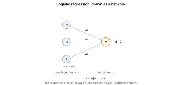 |
| + | |
| + | *Each edge carries one weight and the neuron applies $\sigma$ to the weighted sum. The neuron fixed at $1$ carries the bias: its weight is $w_0$.* |
| + | |
| + | *Remark:* the bias stays folded into the weights throughout this module, drawn as a constant neuron. The [Deep Learning](/en/Deep%20Learning) course instead keeps an explicit bias vector $b^{[l]}$, and flags the change of convention when it introduces it. |
| + | |
| + | ### 6.2.2 Insert a hidden layer |
| + | |
| + | Nothing forces the output neuron to read the raw input. Insert a few neurons between the input and the output, say three. Each one is the same dot-product unit as always, with its own weights $w_i$ and a nonlinear activation $g$: |
| + | |
| + | $$a_i = g(w_i^T x), \qquad i = 1, 2, 3$$ |
| - | $$\boxed{ W^{[2]}\!\left(W^{[1]} x + b^{[1]}\right) + b^{[2]} = W' x + b' }$$ |
| + | Stack the three weight vectors $w_i^T$ as the rows of a matrix $W^{[1]}$ and the whole layer becomes one line, $a = g(W^{[1]} x)$. The bracketed superscript $[1]$ is new, and it exists for a mundane reason: the model now has two sets of weights, so each needs a name. $[l]$ simply says which layer a symbol belongs to. |
| - | so depth would add nothing. The nonlinear activation is what makes stacking worthwhile. |
| + | The output neuron has not changed at all. It is still the logistic regression of section 6.2.1, it just reads the three learned values $a$, augmented with a constant $a_0 = 1$ (every layer gets a bias neuron, exactly like the input), instead of the raw input: |
| - | ## 6.2 Layers: input, hidden, output |
| + | $$\boxed{ \hat{y} = \sigma\!\left(w^{[2]T} a\right) = \sigma\!\left(w^{[2]T}\, g(W^{[1]} x)\right) }$$ |
| - | A single neuron computes $a = g(w^T x + b)$. A layer stacks many neurons, and a network stacks layers. Layer $l$ transforms the previous activations into new ones: |
| + | 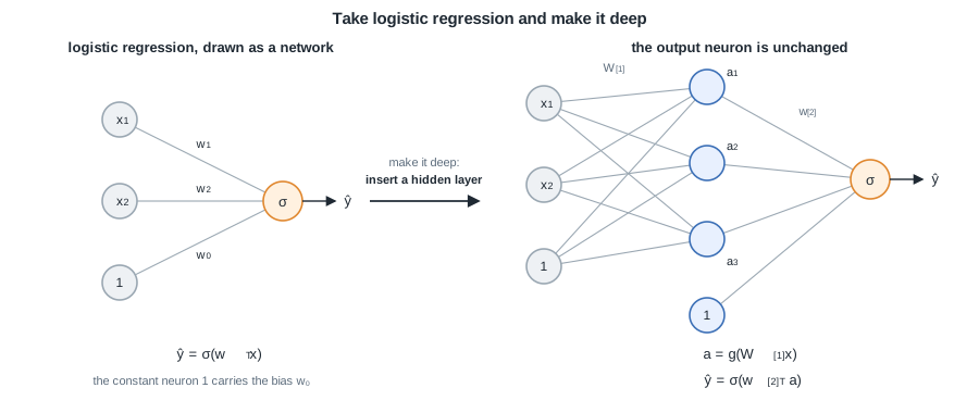 |
| - | $$\boxed{ z^{[l]} = W^{[l]} a^{[l-1]} + b^{[l]}, \quad a^{[l]} = g^{[l]}\!\left(z^{[l]}\right), \quad a^{[0]} = x, \quad \hat{y} = a^{[L]} }$$ |
| + | *The orange output neuron is identical in both drawings. Making the model deep changed what it reads: three learned features $a$ instead of the raw $x$. Each layer carries its own constant neuron $1$, whose outgoing weights are the biases.* |
| - | The input layer holds $x$, the hidden layers learn intermediate features, and the output layer produces the prediction $\hat{y}$. |
| + | Two facts about this insertion carry the whole story. |
| + | |
| + | **The hidden activation must be nonlinear.** If $g$ were the identity, the two layers would collapse into a single linear map, |
| + | |
| + | $$\boxed{ W^{[2]}\!\left(W^{[1]} x\right) = W' x }$$ |
| + | |
| + | and depth would add nothing. The nonlinearity is what makes stacking worthwhile, and it is why XOR is now within reach. |
| + | |
| + | **The hidden layer learns the features.** The output neuron is still a linear classifier, so the hidden layer's job is to move the data somewhere the classes become linearly separable. It plays exactly the role of the basis functions $\phi$ of [Linear regression](/en/Machine%20Learning/04%20Linear%20regression), with one upgrade: $\phi$ was fixed by hand before training, while $a$ is learned from the data, end to end. |
| + | |
| + | ### 6.2.3 How to make a prediction? |
| + | |
| + | One hidden layer worked, so repeat the move: the vector $a^{[1]}$ can feed a second hidden layer, whose output $a^{[2]}$ can feed a third, until an output layer produces $\hat{y}$. Layer $l$ owns its weight matrix $W^{[l]}$ (one row per neuron, so the output layer above had the single row $w^{[2]T}$) and its activation $g^{[l]}$. Width and depth are the capacity dials: more units and more layers mean more parameters and more expressive boundaries, and, as [General concepts](/en/Machine%20Learning/02%20General%20concepts) warned, more room to overfit. |
| 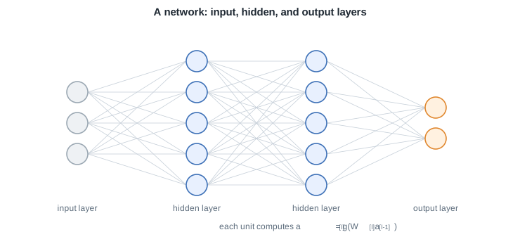 | |
| - | *Each edge carries a weight in $W^{[l]}$ and each unit adds a bias then applies the activation.* |
| + | *Each edge carries a weight in $W^{[l]}$. The constant bias neurons are left out of the drawing.* |
| + | |
| + | Computing the prediction by reading the network left to right is called forward propagation, and the general formula only restates what the last two sections built, once per layer: |
| + | |
| + | $$\boxed{ z^{[l]} = W^{[l]} a^{[l-1]}, \quad a^{[l]} = g^{[l]}\!\left(z^{[l]}\right), \quad a^{[0]} = x, \quad \hat{y} = a^{[L]} }$$ |
| + | |
| + | with one convention to remember: every $a^{[l]}$, like the input, is read with its bias neuron $a^{[l]}_0 = 1$ prepended. In vectorized form the whole mini-batch flows at once, one matrix operation per layer with the examples as columns, which is both clearer and far faster: |
| + | |
| + | $$\boxed{ Z^{[l]} = W^{[l]} A^{[l-1]} }$$ |
| + | |
| + | Forward propagation is the first half of every training step. The second half, backpropagation, runs the same wiring in reverse (section 6.4). |
| + | |
| + | ### 6.2.4 The formula on the graph |
| - | *Remark:* the bias is now written out explicitly and each layer has its own weight matrix $W^{[l]}$, unlike the earlier convention of folding the bias into $\theta^T x$ with $x_0 = 1$. This is the notation the Deep Learning course uses throughout. |
| + | Every symbol in the forward propagation formula lives somewhere on the network drawing. The figure below places each one on the smallest interesting network, two inputs, one hidden layer of two units, and one output: |
| - | ## 6.3 Output layer: binary and multiclass |
| + | 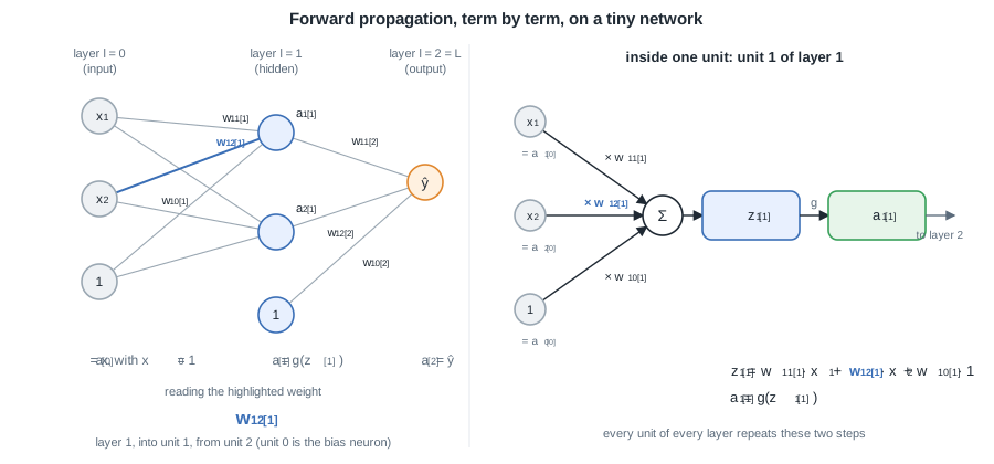 |
| - | The output layer matches the task, reusing the losses from [Linear classification](/en/Machine%20Learning/05%20Linear%20classification). For two classes, a sigmoid output with the binary cross-entropy, and for $k$ classes, a softmax output with the categorical cross-entropy: |
| + | *Left: the superscript $[l]$ names the layer, each edge carries one weight $w^{[l]}_{ij}$, and the neurons fixed at $1$ carry the biases $w^{[l]}_{i0}$. Right: inside a unit, the weighted sum gives $z^{[l]}_i$, then the activation $g$ turns it into $a^{[l]}_i$.* |
| + | |
| + | | Symbol | Name | Where it lives on the graph | |
| + | | --- | --- | --- | |
| + | | $l$, $L$ | layer index, number of layers | which column of units ($l = 0$ is the input, here $L = 2$) | |
| + | | $x = a^{[0]}$ | the input | the leftmost column | |
| + | | $w^{[l]}_{ij}$ | one weight | the number carried by one edge: into unit $i$ of layer $l$, from unit $j$ of layer $l-1$ | |
| + | | $W^{[l]}$ | weight matrix of layer $l$ | all the edges arriving into layer $l$, one row per unit | |
| + | | $x_0$, $a^{[l]}_0$ | bias neuron | a unit fixed at $1$ in each layer, whose outgoing weight $w^{[l]}_{i0}$ is the bias of unit $i$ | |
| + | | $z^{[l]}_i$ | pre-activation | the weighted sum the unit computes before applying $g$ | |
| + | | $g^{[l]}$ | activation function | applied inside every unit of layer $l$ | |
| + | | $a^{[l]}_i$ | activation | the value the unit sends along its outgoing edges | |
| + | | $\hat{y} = a^{[L]}$ | the prediction | what leaves the last layer | |
| + | |
| + | Now run this exact network with numbers. Take $x = (1, 2)$, augmented to $(1, 1, 2)$ by the bias neuron $x_0 = 1$, the sigmoid of the previous module as the activation everywhere, with |
| + | |
| + | $$W^{[1]} = \begin{pmatrix} 0 & 2 & -1 \\ -1 & 1 & 1 \end{pmatrix}, \qquad W^{[2]} = \begin{pmatrix} 0 & 1 & 1 \end{pmatrix}$$ |
| + | |
| + | Row $i$ of $W^{[1]}$ collects the weights of the edges arriving into hidden unit $i$, bias first. Layer 1, unit by unit: |
| + | |
| + | $$z^{[1]}_1 = \underbrace{0}_{w^{[1]}_{10}} \cdot \underbrace{1}_{x_0} + \underbrace{2}_{w^{[1]}_{11}} \cdot \underbrace{1}_{x_1} + \underbrace{(-1)}_{w^{[1]}_{12}} \cdot \underbrace{2}_{x_2} = 0, \qquad a^{[1]}_1 = \sigma(0) = 0.5$$ |
| + | |
| + | $$z^{[1]}_2 = -1 \cdot 1 + 1 \cdot 1 + 1 \cdot 2 = 2, \qquad a^{[1]}_2 = \sigma(2) \approx 0.88$$ |
| + | |
| + | Hidden unit 1 lands exactly on zero, the midpoint of the sigmoid, so it outputs $0.5$, while unit 2 sits high on the curve. The output layer repeats the same two steps, now reading $a^{[1]} = (0.5, 0.88)$, augmented to $(1, 0.5, 0.88)$ by its own bias neuron, instead of $x$: |
| + | |
| + | $$z^{[2]} = 0 \cdot 1 + 1 \cdot 0.5 + 1 \cdot 0.88 = 1.38, \qquad \hat{y} = a^{[2]} = \sigma(1.38) \approx 0.80$$ |
| + | |
| + | The network predicts class 1 with probability about $0.80$. That is all forward propagation does: multiply by the edge weights, bias neuron included, apply the activation, at every unit of every layer. |
| + | |
| + | ## 6.3 The loss function |
| + | |
| + | The network's body is task-agnostic. The task lives in the last layer: its activation shapes $\hat{y}$, and the loss compares $\hat{y}$ to the label, reusing the losses of [General concepts](/en/Machine%20Learning/02%20General%20concepts) and [Linear classification](/en/Machine%20Learning/05%20Linear%20classification): |
| + | |
| + | | Task | Output activation | Loss function | |
| + | | --- | --- | --- | |
| + | | regression | identity | squared error | |
| + | | binary classification | sigmoid | binary cross-entropy | |
| + | | multiclass classification | softmax | categorical cross-entropy | |
| $$\boxed{ \hat{y} = \frac{1}{1 + e^{-z}} \quad\text{(binary)} \qquad \hat{y}_c = \frac{e^{z_c}}{\sum_{j} e^{z_j}} \quad\text{(multiclass)} }$$ | |
| - | ## 6.4 Activation functions and the zero-centered problem |
| + | *Remark:* these are exactly the neuron heads of [Linear classification](/en/Machine%20Learning/05%20Linear%20classification). A network is that same head with learned features underneath instead of raw inputs. |
| + | |
| + | ## 6.4 How to optimize the parameters? |
| + | |
| + | Nothing here is new either: training a network follows the same steps as every model of this course, so let us walk them in order. |
| + | |
| + | **Step 0: pose the objective.** Find the weights that minimize the loss plus a regularizer that keeps them small, the maximum a posteriori recipe of [Linear regression](/en/Machine%20Learning/04%20Linear%20regression): |
| + | |
| + | $$\boxed{ W^\star = \arg\min_W \; L(W) + \lambda\, R(W), \qquad R(W) = \lVert W \rVert_1 \;\text{ or }\; \lVert W \rVert_2^2 }$$ |
| + | |
| + | **Step 1: choose the loss.** That is section 6.3, and its table carries the warning that comes with it: the loss and the output activation are picked as a pair. Cross-entropy calls for a softmax (or a sigmoid), squared error for an identity output. |
| + | |
| + | **Step 2: descend the gradient.** Update every weight by a small step against its gradient, with learning rate $\alpha$, exactly the gradient descent of [Linear classification](/en/Machine%20Learning/05%20Linear%20classification): |
| + | |
| + | $$\boxed{ w^{[l]}_{ij} \leftarrow w^{[l]}_{ij} - \alpha\, \frac{\partial \left(L + \lambda R\right)}{\partial w^{[l]}_{ij}} }$$ |
| + | |
| + | **Step 3: get the gradient by backpropagation.** The genuinely new piece is computing that gradient for every weight in a stack of layers. Backpropagation does it with the chain rule, in one forward and one backward sweep: forward propagation caches each $z^{[l]}$ and $a^{[l]}$, then the backward pass propagates the loss gradient layer by layer, from the output back to the first layer, reusing the cache. With the layer error $\delta^{[l]} = \partial L / \partial z^{[l]}$, |
| + | |
| + | $$\boxed{ \delta^{[l]} = \left((W^{[l+1]})^T \delta^{[l+1]}\right) \odot g'^{[l]}\!\left(z^{[l]}\right), \qquad \frac{\partial L}{\partial W^{[l]}} = \delta^{[l]} (a^{[l-1]})^T }$$ |
| + | |
| + | The bias neurons fit for free: being constant, they receive no error (their row of $(W^{[l+1]})^T \delta^{[l+1]}$ is simply dropped), and since $a^{[l-1]}$ includes the constant $1$, the same outer product delivers the bias gradients along with the rest. |
| - | The hidden activation is usually the sigmoid, the hyperbolic tangent, or the rectified linear unit: |
| + | 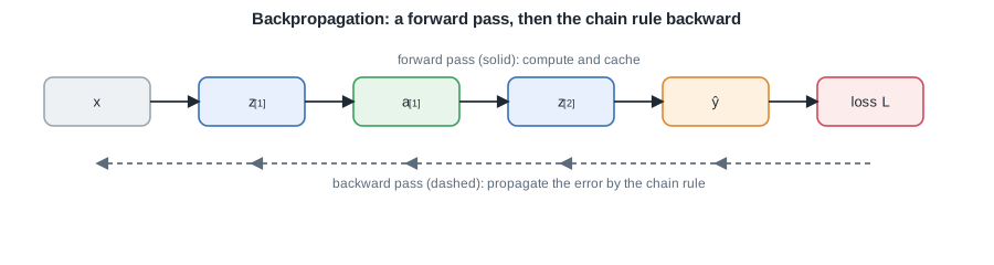 |
| + | |
| + | *Forward propagation computes and caches the activations, backpropagation sends the loss gradient back through the same edges. The [Backpropagation](/en/Deep%20Learning/05%20Backpropagation) lesson of the Deep Learning course derives it step by step.* |
| + | |
| + | <details class="proof"> |
| + | <summary>Full example: one gradient descent step on the tiny network</summary> |
| + | |
| + | Pick up the network of section 6.2.4 exactly where forward propagation left it: $\bar{x} = (1, 1, 2)$, $a^{[1]} = (0.5,\ 0.88)$, $\hat{y} = 0.80$, and give the example a label: the true class is $y = 0$. Take the binary cross-entropy of section 6.3 with no regularization ($\lambda = 0$), so the loss is |
| + | |
| + | $$L = -\ln(1 - \hat{y}) = -\ln(0.20) \approx 1.61$$ |
| + | |
| + | The network is confidently wrong, and the gradient is about to say so. |
| + | |
| + | **Backward through the output layer.** For a sigmoid output trained with cross-entropy, the output error collapses to the familiar $\hat{y} - y$ of [Linear classification](/en/Machine%20Learning/05%20Linear%20classification): |
| + | |
| + | $$\delta^{[2]} = \hat{y} - y = 0.80$$ |
| + | |
| + | Each weight of $W^{[2]}$ receives $\delta^{[2]}$ times the activation it reads (the outer-product formula, bias neuron included): |
| + | |
| + | $$\frac{\partial L}{\partial W^{[2]}} = \delta^{[2]} \left(\bar{a}^{[1]}\right)^T = 0.80 \cdot (1,\ 0.5,\ 0.88) = (0.80,\ 0.40,\ 0.70)$$ |
| + | |
| + | **Backward through the hidden layer.** Each hidden unit takes its share of the error through its outgoing weight, times its own slope $\sigma'(z) = \sigma(z)(1 - \sigma(z))$: |
| + | |
| + | $$\delta^{[1]}_1 = w^{[2]}_{11}\, \delta^{[2]}\, \sigma'(0) = 1 \cdot 0.80 \cdot 0.25 = 0.20, \qquad \delta^{[1]}_2 = 1 \cdot 0.80 \cdot 0.10 = 0.08$$ |
| + | |
| + | (the constant bias neuron takes no error, and note the small slope $0.10$ of unit 2: section 6.5 returns to it). Then the same outer product against $\bar{x} = (1, 1, 2)$: |
| + | |
| + | $$\frac{\partial L}{\partial W^{[1]}} = \delta^{[1]}\, \bar{x}^T = \begin{pmatrix} 0.20 & 0.20 & 0.40 \\ 0.08 & 0.08 & 0.16 \end{pmatrix}$$ |
| + | |
| + | **The update.** Step 2 with a deliberately large $\alpha = 1$, so the movement is visible: |
| + | |
| + | $$W^{[2]} \leftarrow (0,\ 1,\ 1) - (0.80,\ 0.40,\ 0.70) = (-0.80,\ 0.60,\ 0.30)$$ |
| + | |
| + | $$W^{[1]} \leftarrow \begin{pmatrix} 0 & 2 & -1 \\ -1 & 1 & 1 \end{pmatrix} - \begin{pmatrix} 0.20 & 0.20 & 0.40 \\ 0.08 & 0.08 & 0.16 \end{pmatrix} = \begin{pmatrix} -0.20 & 1.80 & -1.40 \\ -1.08 & 0.92 & 0.84 \end{pmatrix}$$ |
| + | |
| + | **Did it help?** Run forward propagation once more with the new weights: $z^{[1]} = (-1.20,\ 1.52)$, $a^{[1]} = (0.23,\ 0.82)$, $z^{[2]} = -0.42$, and |
| + | |
| + | $$\hat{y} = \sigma(-0.42) \approx 0.40, \qquad L = -\ln(1 - 0.40) \approx 0.51$$ |
| + | |
| + | One step, and the prediction for class 1 fell from $0.80$ to $0.40$, the loss from $1.61$ to $0.51$. Training is this loop, repeated over mini-batches until the loss settles. |
| + | |
| + | </details> |
| + | |
| + | ## 6.5 The vanishing gradient |
| + | |
| + | The backpropagation formula hides a trap. Every layer the error crosses multiplies $\delta^{[l]}$ by the local slope $g'(z^{[l]})$, so the gradient reaching layer 1 contains one such factor per layer. With sigmoid activations those factors are small by construction: |
| + | |
| + | $$\boxed{ \sigma'(z) = \sigma(z)\left(1 - \sigma(z)\right) \le \tfrac{1}{4} }$$ |
| + | |
| + | The result is the vanishing gradient: the layers near the output learn, the layers near the input receive almost nothing and barely move. Deep sigmoid networks stall, and the fix is not a better optimizer, it is a better activation (section 6.6). |
| + | |
| + | <details class="proof"> |
| + | <summary>Proof: the gradient shrinks geometrically with depth</summary> |
| + | |
| + | **Step 1: the sigmoid's slope never exceeds $1/4$.** Differentiate $\sigma(z) = (1 + e^{-z})^{-1}$ with the chain rule: |
| + | |
| + | $$\sigma'(z) = \frac{e^{-z}}{\left(1 + e^{-z}\right)^2} = \frac{1}{1 + e^{-z}} \cdot \frac{e^{-z}}{1 + e^{-z}} = \sigma(z)\left(1 - \sigma(z)\right)$$ |
| + | |
| + | Write $s = \sigma(z) \in (0, 1)$. The product $s(1 - s)$ is a downward parabola in $s$, largest at $s = \tfrac{1}{2}$ where it equals $\tfrac{1}{4}$. So the bound holds, with equality only at $z = 0$, and saturation makes it far worse: in the worked example of section 6.2.4, hidden unit 2 sits at $\sigma(2) \approx 0.88$, where the slope has already dropped to $0.88 \cdot 0.12 \approx 0.10$. |
| + | |
| + | **Step 2: backpropagation multiplies those slopes.** Take the simplest deep network, a chain of $L$ layers with one unit each, so every quantity is a scalar. Applying the chain rule from the output back to layer 1, each layer crossed contributes the factor $\partial z^{[l]} / \partial z^{[l-1]} = w^{[l]}\, \sigma'(z^{[l-1]})$: |
| + | |
| + | $$\frac{\partial L}{\partial z^{[1]}} = \frac{\partial L}{\partial z^{[L]}} \prod_{l=2}^{L} w^{[l]}\, \sigma'(z^{[l-1]})$$ |
| + | |
| + | With weights of typical size $|w^{[l]}| \le 1$, every factor is at most $\tfrac{1}{4}$ in absolute value, so |
| + | |
| + | $$\boxed{ \left|\frac{\partial L}{\partial z^{[1]}}\right| \le \left(\tfrac{1}{4}\right)^{L-1} \left|\frac{\partial L}{\partial z^{[L]}}\right| }$$ |
| + | |
| + | Ten layers already shrink the gradient by about $10^{-6}$. The full matrix case is the recursion of section 6.4, with the same conclusion. $\blacksquare$ |
| + | |
| + | </details> |
| + | |
| + | Weights much larger than $1$ only trade the problem for its mirror image, the exploding gradient. The [Initialization and vanishing gradients](/en/Deep%20Learning/07%20Initialization%20and%20vanishing%20gradients) lesson of the Deep Learning course gives the full treatment. |
| + | |
| + | ## 6.6 Activation functions |
| + | |
| + | So which activation should $g$ be? The candidates, in the order history tried them: |
| $$\boxed{ \sigma(z) = \frac{1}{1 + e^{-z}}, \qquad \tanh(z), \qquad \mathrm{ReLU}(z) = \max(0, z) }$$ | |
| - | The sigmoid saturates in its tails, and its outputs are never negative, so a unit's incoming weights all receive gradients of the same sign and the updates zig-zag. The zero-centered $\tanh$ removes that bias, and ReLU avoids positive-side saturation altogether, which is why it is the common default. |
| + | The sigmoid saturates in both tails, which is exactly what section 6.5 punished, and its outputs are never negative, so a unit's incoming weights all receive gradients of the same sign and the updates zig-zag. The zero-centered $\tanh$ removes that bias but still saturates. ReLU keeps a slope of exactly $1$ on its whole positive side, so the shrinking factors of section 6.5 disappear, and it costs almost nothing to compute. That is why it is the default hidden activation today. |
|  | |
| *The tanh is zero-centered while the sigmoid is not, and ReLU stays linear for positive inputs.* | |
| - | ## 6.5 Chain rule and backpropagation |
| + | ReLU has one blind spot: a unit whose input stays negative outputs $0$, has slope $0$, and stops learning, a dead unit. Variants such as Leaky ReLU, $\max(0.01 z, z)$, and ELU keep a small slope on the negative side to prevent it. In practice: start with ReLU, try its variants if units die, and keep the sigmoid only where section 6.3 needs it, at the output of a binary classifier. The [Activation functions](/en/Deep%20Learning/03%20Activation%20functions) lesson of the Deep Learning course compares them all. |
| - | Training minimizes the loss by gradient descent, which needs its gradient with respect to every weight. Backpropagation computes all of them in one forward and one backward sweep: the forward pass caches each $z^{[l]}$ and $a^{[l]}$, then the backward pass applies the chain rule from the loss back to the first layer, reusing the cache. With the layer error $\delta^{[l]} = \partial L / \partial z^{[l]}$, |
| + | ## 6.7 Good practices |
| - | $$\boxed{ \delta^{[l]} = \left((W^{[l+1]})^T \delta^{[l+1]}\right) \odot g'^{[l]}\!\left(z^{[l]}\right), \qquad \frac{\partial L}{\partial W^{[l]}} = \delta^{[l]} (a^{[l-1]})^T }$$ |
| + | Five habits make the difference between a network that trains and one that stalls. |
| - |  |
| + | **Train on mini-batches.** [Linear classification](/en/Machine%20Learning/05%20Linear%20classification) offered two extremes, the full batch or a single example per step. Networks train on mini-batches, a small batch per step: a gradient accurate enough to make progress, a step cheap enough to take thousands of them, and the vectorized forward propagation of section 6.2.3 processes the whole mini-batch in one matrix product per layer. |
| + | |
| + | **Initialize with care.** Equal weights would make every unit of a layer compute the same thing forever, so start small and random to break the symmetry. The scale matters too: too small and the activations shrink toward zero layer after layer, too large and they saturate. Scale the variance by the unit's number of inputs, Xavier for tanh, He for ReLU. |
| + | |
| + | **Center and normalize the inputs.** Standardize each feature (subtract its mean, divide by its standard deviation), so no feature dominates the first dot products and the all-positive-input zig-zag of section 6.6 disappears at the first layer. |
| + | |
| + | **Dropout.** Randomly zero a fraction of units during training so none can lean on its neighbors, a regularizer in the spirit of [General concepts](/en/Machine%20Learning/02%20General%20concepts). At prediction time every unit stays on and outputs are scaled by the keep probability, which approximates averaging the many thinned networks ([Regularization and dropout](/en/Deep%20Learning/09%20Regularization%20and%20dropout)). |
| + | |
| + | **Sanity-check before training long.** A freshly initialized $K$-class classifier should start near the loss $\ln K$ (about $2.3$ for $K = 10$). A tiny training set should be easy to overfit: if the network cannot, the code is broken. Watch the training and validation curves. And since backpropagation is error-prone, check its analytic gradient against a numerical finite-difference estimate: |
| + | |
| + | $$\boxed{ \frac{\partial L}{\partial w} \approx \frac{L(w + \varepsilon) - L(w - \varepsilon)}{2\varepsilon} }$$ |
| + | |
| + | ## 6.8 Gradient descent, improved |
| + | |
| + | Plain gradient descent takes the steepest step and nothing more, and three landscapes defeat it: plateaus, where the slope is nearly zero and progress stalls, saddle points (common in high dimension), where the gradient is exactly zero without being a minimum, and ravines, steep in one direction and shallow in another, where the step oscillates across the walls while crawling along the floor. |
| - | *The [Backpropagation](/en/Deep%20Learning/05%20Backpropagation) lesson of the Deep Learning course derives this step by step.* |
| + | **Momentum** treats the update as a velocity with friction: gradients accumulate, persistent directions build up speed, oscillating ones cancel out: |
| - | ## 6.6 Training in practice |
| + | $$\boxed{ v \leftarrow \rho\, v + \nabla_W L, \qquad W \leftarrow W - \alpha\, v }$$ |
| - | - **Mini-batches.** Estimate the gradient on a small batch of examples at a time, a middle ground between the full batch (accurate but slow) and one example (noisy but cheap). |
| - | - **Vanishing gradient.** Through many saturating layers the backpropagated gradient is a product of small factors and shrinks toward zero, so early layers barely learn. ReLU activations and careful initialization keep it alive. |
| - | - **Initialization.** Start the weights small and random to break symmetry, scaling the variance by the number of inputs (Xavier or He), so signals neither vanish nor explode through depth. |
| - | - **Dropout.** Randomly zero a fraction of units during training. This prevents units from co-adapting and acts as a regularizer, in the spirit of the regularization of [General concepts](/en/Machine%20Learning/02%20General%20concepts). |
| + | with the friction $\rho$ typically around $0.9$. |
| - | ## 6.7 Sanity checks and vectorization |
| + | **RMSProp** gives each parameter its own step size, dividing by a running average of the gradient's magnitude, so steep directions are tamed and flat ones sped up: |
| - | Backpropagation is error-prone, so check the analytic gradient against a numerical finite-difference estimate: |
| + | $$\boxed{ m \leftarrow \beta\, m + (1 - \beta) \left(\nabla_W L\right)^2, \qquad W \leftarrow W - \frac{\alpha}{\sqrt{m} + \varepsilon}\, \nabla_W L }$$ |
| - | $$\boxed{ \frac{\partial L}{\partial \theta} \approx \frac{L(\theta + \varepsilon) - L(\theta - \varepsilon)}{2\varepsilon} }$$ |
| + | **Adam** combines the two ideas, a velocity for the direction and a per-parameter scale for the step (the full version also corrects a startup bias in $v$ and $m$), and is the default optimizer in practice: |
| - | and implement the passes in vectorized form, one matrix operation per layer over the whole mini-batch (columns are examples), which is both clearer and far faster: |
| + | $$\boxed{ v \leftarrow \beta_1 v + (1 - \beta_1)\, \nabla_W L, \qquad m \leftarrow \beta_2 m + (1 - \beta_2) \left(\nabla_W L\right)^2, \qquad W \leftarrow W - \alpha\, \frac{v}{\sqrt{m} + \varepsilon} }$$ |
| - | $$\boxed{ Z^{[l]} = W^{[l]} A^{[l-1]} + b^{[l]} }$$ |
| + | Two habits complete the picture: decay the learning rate as training advances, and remember that all three methods still consume the mini-batch gradients of section 6.7, they only spend them more wisely. The [Optimization](/en/Deep%20Learning/06%20Optimization) lesson of the Deep Learning course derives each one and adds the learning-rate schedules. |
| *This module is the doorway to the [Deep Learning](/en/Deep%20Learning) course, which develops architectures, optimizers, initialization, normalization, and regularization in full. The next module returns to linear models from a new angle, the maximum-margin classifier.* | |
| /dev/null .. en/Machine Learning/06 Multilayer neural networks/forward-notation.svg | |
| @@ 0,0 1,96 @@ | |
| + | <svg xmlns="http://www.w3.org/2000/svg" viewBox="0 0 900 420" width="900" height="420" font-family="Helvetica, Arial, sans-serif"> |
| + | <defs> |
| + | <marker id="arrow" viewBox="0 0 10 10" refX="8.5" refY="5" markerWidth="7" markerHeight="7" orient="auto-start-reverse"><path d="M0 0L10 5L0 10z" fill="#1f2933"/></marker> |
| + | <marker id="arrowmuted" viewBox="0 0 10 10" refX="8.5" refY="5" markerWidth="7" markerHeight="7" orient="auto-start-reverse"><path d="M0 0L10 5L0 10z" fill="#5b6b7b"/></marker> |
| + | </defs> |
| + | <rect width="900" height="420" fill="#ffffff"/> |
| + | <text x="450" y="22" font-size="15" font-weight="600" fill="#1f2933" text-anchor="middle">Forward propagation, term by term, on a tiny network</text> |
| + | |
| + | <!-- Panel A: annotated network --> |
| + | <text x="90" y="52" font-size="11" fill="#5b6b7b" text-anchor="middle">layer l = 0</text> |
| + | <text x="90" y="66" font-size="11" fill="#5b6b7b" text-anchor="middle">(input)</text> |
| + | <text x="250" y="52" font-size="11" fill="#5b6b7b" text-anchor="middle">layer l = 1</text> |
| + | <text x="250" y="66" font-size="11" fill="#5b6b7b" text-anchor="middle">(hidden)</text> |
| + | <text x="385" y="52" font-size="11" fill="#5b6b7b" text-anchor="middle">layer l = 2 = L</text> |
| + | <text x="385" y="66" font-size="11" fill="#5b6b7b" text-anchor="middle">(output)</text> |
| + | |
| + | <line x1="105.9" y1="106.5" x2="234.1" y2="118.5" stroke="#9aa7b2" stroke-width="1.1"/> |
| + | <line x1="103.4" y1="113.8" x2="236.6" y2="201.2" stroke="#9aa7b2" stroke-width="1.1"/> |
| + | <line x1="105.7" y1="182.9" x2="234.3" y2="207.1" stroke="#9aa7b2" stroke-width="1.1"/> |
| + | <line x1="105" y1="174.4" x2="235" y2="125.6" stroke="#3b6fb6" stroke-width="2"/> |
| + | <line x1="102.2" y1="244.7" x2="237.8" y2="130.3" stroke="#9aa7b2" stroke-width="1.1"/> |
| + | <line x1="105.4" y1="250.7" x2="234.6" y2="214.3" stroke="#9aa7b2" stroke-width="1.1"/> |
| + | <line x1="265.2" y1="125.1" x2="369.8" y2="159.9" stroke="#9aa7b2" stroke-width="1.1"/> |
| + | <line x1="265.2" y1="204.9" x2="369.8" y2="170.1" stroke="#9aa7b2" stroke-width="1.1"/> |
| + | <line x1="262" y1="274.4" x2="373" y2="175.6" stroke="#9aa7b2" stroke-width="1.1"/> |
| + | |
| + | <text x="205" y="110" font-size="11" fill="#1f2933" text-anchor="middle">w<tspan baseline-shift="sub" font-size="8px">11</tspan><tspan baseline-shift="super" font-size="8px">[1]</tspan></text> |
| + | <text x="200" y="132" font-size="11" font-weight="600" fill="#3b6fb6" text-anchor="middle">w<tspan baseline-shift="sub" font-size="8px">12</tspan><tspan baseline-shift="super" font-size="8px">[1]</tspan></text> |
| + | <text x="150" y="185" font-size="11" fill="#1f2933" text-anchor="middle">w<tspan baseline-shift="sub" font-size="8px">10</tspan><tspan baseline-shift="super" font-size="8px">[1]</tspan></text> |
| + | <text x="322" y="131" font-size="11" fill="#1f2933" text-anchor="middle">w<tspan baseline-shift="sub" font-size="8px">11</tspan><tspan baseline-shift="super" font-size="8px">[2]</tspan></text> |
| + | <text x="300" y="214" font-size="11" fill="#1f2933" text-anchor="middle">w<tspan baseline-shift="sub" font-size="8px">12</tspan><tspan baseline-shift="super" font-size="8px">[2]</tspan></text> |
| + | <text x="332" y="241" font-size="11" fill="#1f2933" text-anchor="middle">w<tspan baseline-shift="sub" font-size="8px">10</tspan><tspan baseline-shift="super" font-size="8px">[2]</tspan></text> |
| + | |
| + | <circle cx="90" cy="105" r="16" fill="#eef1f4" stroke="#9aa7b2" stroke-width="1.6"/> |
| + | <text x="90" y="109" font-size="12" fill="#1f2933" text-anchor="middle">x<tspan baseline-shift="sub" font-size="9px">1</tspan></text> |
| + | <circle cx="90" cy="180" r="16" fill="#eef1f4" stroke="#9aa7b2" stroke-width="1.6"/> |
| + | <text x="90" y="184" font-size="12" fill="#1f2933" text-anchor="middle">x<tspan baseline-shift="sub" font-size="9px">2</tspan></text> |
| + | <circle cx="90" cy="255" r="16" fill="#eef1f4" stroke="#9aa7b2" stroke-width="1.6"/> |
| + | <text x="90" y="259" font-size="12" fill="#1f2933" text-anchor="middle">1</text> |
| + | <circle cx="250" cy="120" r="16" fill="#e8f0fe" stroke="#3b6fb6" stroke-width="1.6"/> |
| + | <circle cx="250" cy="210" r="16" fill="#e8f0fe" stroke="#3b6fb6" stroke-width="1.6"/> |
| + | <circle cx="250" cy="285" r="16" fill="#e8f0fe" stroke="#3b6fb6" stroke-width="1.6"/> |
| + | <text x="250" y="289" font-size="12" fill="#1f2933" text-anchor="middle">1</text> |
| + | <circle cx="385" cy="165" r="16" fill="#fff1e0" stroke="#e0872e" stroke-width="1.6"/> |
| + | <text x="385" y="170" font-size="13" fill="#1f2933" text-anchor="middle">ŷ</text> |
| + | |
| + | <text x="268" y="106" font-size="11" fill="#1f2933">a<tspan baseline-shift="sub" font-size="8px">1</tspan><tspan baseline-shift="super" font-size="8px">[1]</tspan></text> |
| + | <text x="268" y="192" font-size="11" fill="#1f2933">a<tspan baseline-shift="sub" font-size="8px">2</tspan><tspan baseline-shift="super" font-size="8px">[1]</tspan></text> |
| + | |
| + | <text x="90" y="330" font-size="12" fill="#5b6b7b" text-anchor="middle">a<tspan baseline-shift="super" font-size="9px">[0]</tspan> = x, with x<tspan baseline-shift="sub" font-size="9px">0</tspan> = 1</text> |
| + | <text x="250" y="330" font-size="12" fill="#5b6b7b" text-anchor="middle">a<tspan baseline-shift="super" font-size="9px">[1]</tspan> = g(z<tspan baseline-shift="super" font-size="9px">[1]</tspan>)</text> |
| + | <text x="385" y="330" font-size="12" fill="#5b6b7b" text-anchor="middle">a<tspan baseline-shift="super" font-size="9px">[2]</tspan> = ŷ</text> |
| + | |
| + | <text x="220" y="358" font-size="11" fill="#5b6b7b" text-anchor="middle">reading the highlighted weight</text> |
| + | <text x="220" y="384" font-size="17" font-weight="600" fill="#3b6fb6" text-anchor="middle">w<tspan baseline-shift="sub" font-size="11px">12</tspan><tspan baseline-shift="super" font-size="11px">[1]</tspan></text> |
| + | <text x="220" y="404" font-size="11" fill="#5b6b7b" text-anchor="middle">layer 1, into unit 1, from unit 2 (unit 0 is the bias neuron)</text> |
| + | |
| + | <line x1="425" y1="40" x2="425" y2="405" stroke="#e3e8ee" stroke-width="1"/> |
| + | |
| + | <!-- Panel B: inside one unit --> |
| + | <text x="665" y="56" font-size="13" font-weight="600" fill="#1f2933" text-anchor="middle">inside one unit: unit 1 of layer 1</text> |
| + | |
| + | <line x1="491.4" y1="118.1" x2="585.3" y2="184.6" stroke="#1f2933" stroke-width="1.4" marker-end="url(#arrow)"/> |
| + | <line x1="494" y1="195" x2="582" y2="195" stroke="#1f2933" stroke-width="1.4" marker-end="url(#arrow)"/> |
| + | <line x1="491.4" y1="271.9" x2="585.3" y2="205.4" stroke="#1f2933" stroke-width="1.4" marker-end="url(#arrow)"/> |
| + | <text x="556" y="146" font-size="11" fill="#1f2933" text-anchor="middle">× w<tspan baseline-shift="sub" font-size="8px">11</tspan><tspan baseline-shift="super" font-size="8px">[1]</tspan></text> |
| + | <text x="538" y="187" font-size="11" font-weight="600" fill="#3b6fb6" text-anchor="middle">× w<tspan baseline-shift="sub" font-size="8px">12</tspan><tspan baseline-shift="super" font-size="8px">[1]</tspan></text> |
| + | <text x="556" y="254" font-size="11" fill="#1f2933" text-anchor="middle">× w<tspan baseline-shift="sub" font-size="8px">10</tspan><tspan baseline-shift="super" font-size="8px">[1]</tspan></text> |
| + | |
| + | <circle cx="480" cy="110" r="14" fill="#eef1f4" stroke="#9aa7b2" stroke-width="1.6"/> |
| + | <text x="480" y="114" font-size="11" fill="#1f2933" text-anchor="middle">x<tspan baseline-shift="sub" font-size="8px">1</tspan></text> |
| + | <text x="480" y="142" font-size="10" fill="#5b6b7b" text-anchor="middle">= a<tspan baseline-shift="sub" font-size="7px">1</tspan><tspan baseline-shift="super" font-size="7px">[0]</tspan></text> |
| + | <circle cx="480" cy="195" r="14" fill="#eef1f4" stroke="#9aa7b2" stroke-width="1.6"/> |
| + | <text x="480" y="199" font-size="11" fill="#1f2933" text-anchor="middle">x<tspan baseline-shift="sub" font-size="8px">2</tspan></text> |
| + | <text x="480" y="227" font-size="10" fill="#5b6b7b" text-anchor="middle">= a<tspan baseline-shift="sub" font-size="7px">2</tspan><tspan baseline-shift="super" font-size="7px">[0]</tspan></text> |
| + | <circle cx="480" cy="280" r="14" fill="#eef1f4" stroke="#9aa7b2" stroke-width="1.6"/> |
| + | <text x="480" y="284" font-size="11" fill="#1f2933" text-anchor="middle">1</text> |
| + | <text x="480" y="312" font-size="10" fill="#5b6b7b" text-anchor="middle">= a<tspan baseline-shift="sub" font-size="7px">0</tspan><tspan baseline-shift="super" font-size="7px">[0]</tspan></text> |
| + | |
| + | <circle cx="600" cy="195" r="18" fill="#ffffff" stroke="#1f2933" stroke-width="1.6"/> |
| + | <text x="600" y="200" font-size="14" fill="#1f2933" text-anchor="middle">Σ</text> |
| + | |
| + | <line x1="618" y1="195" x2="636" y2="195" stroke="#1f2933" stroke-width="1.4" marker-end="url(#arrow)"/> |
| + | <rect x="636" y="173" width="88" height="44" rx="8" fill="#e8f0fe" stroke="#3b6fb6" stroke-width="1.6"/> |
| + | <text x="680" y="199" font-size="13" fill="#1f2933" text-anchor="middle">z<tspan baseline-shift="sub" font-size="9px">1</tspan><tspan baseline-shift="super" font-size="9px">[1]</tspan></text> |
| + | <line x1="724" y1="195" x2="750" y2="195" stroke="#1f2933" stroke-width="1.4" marker-end="url(#arrow)"/> |
| + | <text x="737" y="187" font-size="11" fill="#5b6b7b" text-anchor="middle">g</text> |
| + | <rect x="750" y="173" width="88" height="44" rx="8" fill="#e7f5ea" stroke="#38a05a" stroke-width="1.6"/> |
| + | <text x="794" y="199" font-size="13" fill="#1f2933" text-anchor="middle">a<tspan baseline-shift="sub" font-size="9px">1</tspan><tspan baseline-shift="super" font-size="9px">[1]</tspan></text> |
| + | <line x1="838" y1="195" x2="864" y2="195" stroke="#5b6b7b" stroke-width="1.3" marker-end="url(#arrowmuted)"/> |
| + | <text x="851" y="216" font-size="10" fill="#5b6b7b" text-anchor="middle">to layer 2</text> |
| + | |
| + | <text x="665" y="340" font-size="13" fill="#1f2933" text-anchor="middle">z<tspan baseline-shift="sub" font-size="9px">1</tspan><tspan baseline-shift="super" font-size="9px">[1]</tspan> = w<tspan baseline-shift="sub" font-size="9px">11</tspan><tspan baseline-shift="super" font-size="9px">[1]</tspan> · x<tspan baseline-shift="sub" font-size="9px">1</tspan> + <tspan font-weight="600" fill="#3b6fb6">w<tspan baseline-shift="sub" font-size="9px">12</tspan><tspan baseline-shift="super" font-size="9px">[1]</tspan></tspan> · x<tspan baseline-shift="sub" font-size="9px">2</tspan> + w<tspan baseline-shift="sub" font-size="9px">10</tspan><tspan baseline-shift="super" font-size="9px">[1]</tspan> · 1</text> |
| + | <text x="665" y="364" font-size="13" fill="#1f2933" text-anchor="middle">a<tspan baseline-shift="sub" font-size="9px">1</tspan><tspan baseline-shift="super" font-size="9px">[1]</tspan> = g(z<tspan baseline-shift="sub" font-size="9px">1</tspan><tspan baseline-shift="super" font-size="9px">[1]</tspan>)</text> |
| + | <text x="665" y="396" font-size="11" fill="#5b6b7b" text-anchor="middle">every unit of every layer repeats these two steps</text> |
| + | </svg> |
| /dev/null .. en/Machine Learning/06 Multilayer neural networks/logreg-network.svg | |
| @@ 0,0 1,32 @@ | |
| + | <svg xmlns="http://www.w3.org/2000/svg" viewBox="0 0 740 345" width="740" height="345" font-family="Helvetica, Arial, sans-serif"> |
| + | <defs> |
| + | <marker id="arrow" viewBox="0 0 10 10" refX="8.5" refY="5" markerWidth="7" markerHeight="7" orient="auto-start-reverse"><path d="M0 0L10 5L0 10z" fill="#1f2933"/></marker> |
| + | </defs> |
| + | <rect width="740" height="345" fill="#ffffff"/> |
| + | <text x="370" y="22" font-size="15" font-weight="600" fill="#1f2933" text-anchor="middle">Logistic regression, drawn as a network</text> |
| + | |
| + | <line x1="284.7" y1="106.4" x2="413.5" y2="162.8" stroke="#9aa7b2" stroke-width="1.1"/> |
| + | <line x1="286" y1="170" x2="412" y2="170" stroke="#9aa7b2" stroke-width="1.1"/> |
| + | <line x1="284.7" y1="233.6" x2="413.5" y2="177.2" stroke="#9aa7b2" stroke-width="1.1"/> |
| + | <text x="349" y="124" font-size="11" fill="#1f2933" text-anchor="middle">w<tspan baseline-shift="sub" font-size="8px">1</tspan></text> |
| + | <text x="349" y="162" font-size="11" fill="#1f2933" text-anchor="middle">w<tspan baseline-shift="sub" font-size="8px">2</tspan></text> |
| + | <text x="349" y="222" font-size="11" fill="#1f2933" text-anchor="middle">w<tspan baseline-shift="sub" font-size="8px">0</tspan></text> |
| + | |
| + | <circle cx="270" cy="100" r="16" fill="#eef1f4" stroke="#9aa7b2" stroke-width="1.6"/> |
| + | <text x="270" y="104" font-size="12" fill="#1f2933" text-anchor="middle">x<tspan baseline-shift="sub" font-size="9px">1</tspan></text> |
| + | <circle cx="270" cy="170" r="16" fill="#eef1f4" stroke="#9aa7b2" stroke-width="1.6"/> |
| + | <text x="270" y="174" font-size="12" fill="#1f2933" text-anchor="middle">x<tspan baseline-shift="sub" font-size="9px">2</tspan></text> |
| + | <circle cx="270" cy="240" r="16" fill="#eef1f4" stroke="#9aa7b2" stroke-width="1.6"/> |
| + | <text x="270" y="244" font-size="12" fill="#1f2933" text-anchor="middle">1</text> |
| + | <text x="270" y="272" font-size="10" fill="#5b6b7b" text-anchor="middle">x<tspan baseline-shift="sub" font-size="7px">0</tspan> = 1 (bias)</text> |
| + | <circle cx="430" cy="170" r="18" fill="#fff1e0" stroke="#e0872e" stroke-width="1.6"/> |
| + | <text x="430" y="175" font-size="13" fill="#1f2933" text-anchor="middle">σ</text> |
| + | <line x1="448" y1="170" x2="478" y2="170" stroke="#1f2933" stroke-width="1.4" marker-end="url(#arrow)"/> |
| + | <text x="490" y="174" font-size="13" fill="#1f2933" text-anchor="middle">ŷ</text> |
| + | |
| + | <text x="270" y="298" font-size="12" fill="#5b6b7b" text-anchor="middle">input layer: holds x</text> |
| + | <text x="430" y="298" font-size="12" fill="#5b6b7b" text-anchor="middle">output neuron</text> |
| + | |
| + | <text x="370" y="322" font-size="13" fill="#1f2933" text-anchor="middle">ŷ = σ(w<tspan baseline-shift="super" font-size="9px">T</tspan>x)</text> |
| + | <text x="370" y="340" font-size="11" fill="#5b6b7b" text-anchor="middle">one neuron: dot product, activation. The constant neuron 1 carries the bias w₀</text> |
| + | </svg> |
| /dev/null .. en/Machine Learning/06 Multilayer neural networks/make-it-deep.svg | |
| @@ 0,0 1,80 @@ | |
| + | <svg xmlns="http://www.w3.org/2000/svg" viewBox="0 0 900 380" width="900" height="380" font-family="Helvetica, Arial, sans-serif"> |
| + | <defs> |
| + | <marker id="arrow" viewBox="0 0 10 10" refX="8.5" refY="5" markerWidth="7" markerHeight="7" orient="auto-start-reverse"><path d="M0 0L10 5L0 10z" fill="#1f2933"/></marker> |
| + | </defs> |
| + | <rect width="900" height="380" fill="#ffffff"/> |
| + | <text x="450" y="22" font-size="15" font-weight="600" fill="#1f2933" text-anchor="middle">Take logistic regression and make it deep</text> |
| + | |
| + | <!-- Panel 1: logistic regression as a network --> |
| + | <text x="185" y="48" font-size="13" font-weight="600" fill="#1f2933" text-anchor="middle">logistic regression, drawn as a network</text> |
| + | |
| + | <line x1="124.3" y1="117.2" x2="243.9" y2="177" stroke="#9aa7b2" stroke-width="1.1"/> |
| + | <line x1="126" y1="185" x2="242" y2="185" stroke="#9aa7b2" stroke-width="1.1"/> |
| + | <line x1="124.3" y1="252.8" x2="243.9" y2="193" stroke="#9aa7b2" stroke-width="1.1"/> |
| + | <text x="184" y="136" font-size="11" fill="#1f2933" text-anchor="middle">w<tspan baseline-shift="sub" font-size="8px">1</tspan></text> |
| + | <text x="184" y="177" font-size="11" fill="#1f2933" text-anchor="middle">w<tspan baseline-shift="sub" font-size="8px">2</tspan></text> |
| + | <text x="184" y="238" font-size="11" fill="#1f2933" text-anchor="middle">w<tspan baseline-shift="sub" font-size="8px">0</tspan></text> |
| + | |
| + | <circle cx="110" cy="110" r="16" fill="#eef1f4" stroke="#9aa7b2" stroke-width="1.6"/> |
| + | <text x="110" y="114" font-size="12" fill="#1f2933" text-anchor="middle">x<tspan baseline-shift="sub" font-size="9px">1</tspan></text> |
| + | <circle cx="110" cy="185" r="16" fill="#eef1f4" stroke="#9aa7b2" stroke-width="1.6"/> |
| + | <text x="110" y="189" font-size="12" fill="#1f2933" text-anchor="middle">x<tspan baseline-shift="sub" font-size="9px">2</tspan></text> |
| + | <circle cx="110" cy="260" r="16" fill="#eef1f4" stroke="#9aa7b2" stroke-width="1.6"/> |
| + | <text x="110" y="264" font-size="12" fill="#1f2933" text-anchor="middle">1</text> |
| + | <circle cx="260" cy="185" r="18" fill="#fff1e0" stroke="#e0872e" stroke-width="1.6"/> |
| + | <text x="260" y="190" font-size="13" fill="#1f2933" text-anchor="middle">σ</text> |
| + | <line x1="278" y1="185" x2="308" y2="185" stroke="#1f2933" stroke-width="1.4" marker-end="url(#arrow)"/> |
| + | <text x="320" y="189" font-size="13" fill="#1f2933" text-anchor="middle">ŷ</text> |
| + | |
| + | <text x="185" y="330" font-size="13" fill="#1f2933" text-anchor="middle">ŷ = σ(w<tspan baseline-shift="super" font-size="9px">T</tspan>x)</text> |
| + | <text x="185" y="354" font-size="11" fill="#5b6b7b" text-anchor="middle">the constant neuron 1 carries the bias w₀</text> |
| + | |
| + | <!-- Transition arrow --> |
| + | <text x="390" y="153" font-size="11" fill="#5b6b7b" text-anchor="middle">make it deep:</text> |
| + | <text x="390" y="169" font-size="11" font-weight="600" fill="#1f2933" text-anchor="middle">insert a hidden layer</text> |
| + | <line x1="340" y1="185" x2="440" y2="185" stroke="#1f2933" stroke-width="1.7" marker-end="url(#arrow)"/> |
| + | |
| + | <!-- Panel 2: hidden layer inserted --> |
| + | <text x="680" y="48" font-size="13" font-weight="600" fill="#1f2933" text-anchor="middle">the output neuron is unchanged</text> |
| + | |
| + | <line x1="515.9" y1="93.4" x2="634.1" y2="81.6" stroke="#9aa7b2" stroke-width="1.1"/> |
| + | <line x1="515" y1="100.5" x2="635" y2="144.5" stroke="#9aa7b2" stroke-width="1.1"/> |
| + | <line x1="512.3" y1="105.2" x2="637.7" y2="209.8" stroke="#9aa7b2" stroke-width="1.1"/> |
| + | <line x1="513.7" y1="161.8" x2="636.3" y2="88.2" stroke="#9aa7b2" stroke-width="1.1"/> |
| + | <line x1="515.9" y1="167.9" x2="634.1" y2="152.1" stroke="#9aa7b2" stroke-width="1.1"/> |
| + | <line x1="515.2" y1="175.1" x2="634.8" y2="214.9" stroke="#9aa7b2" stroke-width="1.1"/> |
| + | <line x1="510.8" y1="233.2" x2="639.2" y2="91.8" stroke="#9aa7b2" stroke-width="1.1"/> |
| + | <line x1="513.5" y1="236.4" x2="636.5" y2="158.6" stroke="#9aa7b2" stroke-width="1.1"/> |
| + | <line x1="515.8" y1="242.4" x2="634.2" y2="222.6" stroke="#9aa7b2" stroke-width="1.1"/> |
| + | <line x1="663.9" y1="88.9" x2="784.3" y2="156.1" stroke="#9aa7b2" stroke-width="1.1"/> |
| + | <line x1="665.9" y1="151.6" x2="782.1" y2="163.2" stroke="#9aa7b2" stroke-width="1.1"/> |
| + | <line x1="665" y1="214.5" x2="783.1" y2="171.2" stroke="#9aa7b2" stroke-width="1.1"/> |
| + | <line x1="662.3" y1="279.8" x2="786.2" y2="176.5" stroke="#9aa7b2" stroke-width="1.1"/> |
| + | |
| + | <text x="560" y="66" font-size="11" fill="#5b6b7b" text-anchor="middle">W<tspan baseline-shift="super" font-size="8px">[1]</tspan></text> |
| + | <text x="738" y="106" font-size="11" fill="#5b6b7b" text-anchor="middle">w<tspan baseline-shift="super" font-size="8px">[2]</tspan></text> |
| + | |
| + | <circle cx="500" cy="95" r="16" fill="#eef1f4" stroke="#9aa7b2" stroke-width="1.6"/> |
| + | <text x="500" y="99" font-size="12" fill="#1f2933" text-anchor="middle">x<tspan baseline-shift="sub" font-size="9px">1</tspan></text> |
| + | <circle cx="500" cy="170" r="16" fill="#eef1f4" stroke="#9aa7b2" stroke-width="1.6"/> |
| + | <text x="500" y="174" font-size="12" fill="#1f2933" text-anchor="middle">x<tspan baseline-shift="sub" font-size="9px">2</tspan></text> |
| + | <circle cx="500" cy="245" r="16" fill="#eef1f4" stroke="#9aa7b2" stroke-width="1.6"/> |
| + | <text x="500" y="249" font-size="12" fill="#1f2933" text-anchor="middle">1</text> |
| + | <circle cx="650" cy="80" r="16" fill="#e8f0fe" stroke="#3b6fb6" stroke-width="1.6"/> |
| + | <circle cx="650" cy="150" r="16" fill="#e8f0fe" stroke="#3b6fb6" stroke-width="1.6"/> |
| + | <circle cx="650" cy="220" r="16" fill="#e8f0fe" stroke="#3b6fb6" stroke-width="1.6"/> |
| + | <circle cx="650" cy="290" r="16" fill="#e8f0fe" stroke="#3b6fb6" stroke-width="1.6"/> |
| + | <text x="650" y="294" font-size="12" fill="#1f2933" text-anchor="middle">1</text> |
| + | <circle cx="800" cy="165" r="18" fill="#fff1e0" stroke="#e0872e" stroke-width="1.6"/> |
| + | <text x="800" y="170" font-size="13" fill="#1f2933" text-anchor="middle">σ</text> |
| + | |
| + | <text x="668" y="70" font-size="11" fill="#1f2933">a<tspan baseline-shift="sub" font-size="8px">1</tspan></text> |
| + | <text x="668" y="138" font-size="11" fill="#1f2933">a<tspan baseline-shift="sub" font-size="8px">2</tspan></text> |
| + | <text x="668" y="244" font-size="11" fill="#1f2933">a<tspan baseline-shift="sub" font-size="8px">3</tspan></text> |
| + | |
| + | <line x1="818" y1="165" x2="848" y2="165" stroke="#1f2933" stroke-width="1.4" marker-end="url(#arrow)"/> |
| + | <text x="860" y="169" font-size="13" fill="#1f2933" text-anchor="middle">ŷ</text> |
| + | |
| + | <text x="670" y="330" font-size="13" fill="#1f2933" text-anchor="middle">a = g(W<tspan baseline-shift="super" font-size="9px">[1]</tspan>x)</text> |
| + | <text x="670" y="354" font-size="13" fill="#1f2933" text-anchor="middle">ŷ = σ(w<tspan baseline-shift="super" font-size="9px">[2]T</tspan>a)</text> |
| + | </svg> |
| en/Machine Learning/06 Multilayer neural networks/mlp-layers.svg .. | |
| @@ 1,1 1,1 @@ | |
| - | <svg xmlns="http://www.w3.org/2000/svg" viewBox="0 0 740 347" width="740" height="347" font-family="Helvetica, Arial, sans-serif"><defs><marker id="arrow" viewBox="0 0 10 10" refX="8.5" refY="5" markerWidth="7" markerHeight="7" orient="auto-start-reverse"><path d="M0 0L10 5L0 10z" fill="#1f2933"/></marker><marker id="arrowmuted" viewBox="0 0 10 10" refX="8.5" refY="5" markerWidth="7" markerHeight="7" orient="auto-start-reverse"><path d="M0 0L10 5L0 10z" fill="#5b6b7b"/></marker></defs><rect width="740" height="347" fill="#ffffff"/><text x="370.0" y="22.0" font-family="Helvetica, Arial, sans-serif" font-size="15" font-weight="600" fill="#1f2933" text-anchor="middle">A network: input, hidden, and output layers</text><line x1="125.0" y1="131.0" x2="265.0" y2="87.0" stroke="#c7d0d9" stroke-width="0.8"/><line x1="125.0" y1="131.0" x2="265.0" y2="131.0" stroke="#c7d0d9" stroke-width="0.8"/><line x1="125.0" y1="131.0" x2="265.0" y2="175.0" stroke="#c7d0d9" stroke-width="0.8"/><line x1="125.0" y1="131.0" x2="265.0" y2="219.0" stroke="#c7d0d9" stroke-width="0.8"/><line x1="125.0" y1="131.0" x2="265.0" y2="263.0" stroke="#c7d0d9" stroke-width="0.8"/><line x1="125.0" y1="175.0" x2="265.0" y2="87.0" stroke="#c7d0d9" stroke-width="0.8"/><line x1="125.0" y1="175.0" x2="265.0" y2="131.0" stroke="#c7d0d9" stroke-width="0.8"/><line x1="125.0" y1="175.0" x2="265.0" y2="175.0" stroke="#c7d0d9" stroke-width="0.8"/><line x1="125.0" y1="175.0" x2="265.0" y2="219.0" stroke="#c7d0d9" stroke-width="0.8"/><line x1="125.0" y1="175.0" x2="265.0" y2="263.0" stroke="#c7d0d9" stroke-width="0.8"/><line x1="125.0" y1="219.0" x2="265.0" y2="87.0" stroke="#c7d0d9" stroke-width="0.8"/><line x1="125.0" y1="219.0" x2="265.0" y2="131.0" stroke="#c7d0d9" stroke-width="0.8"/><line x1="125.0" y1="219.0" x2="265.0" y2="175.0" stroke="#c7d0d9" stroke-width="0.8"/><line x1="125.0" y1="219.0" x2="265.0" y2="219.0" stroke="#c7d0d9" stroke-width="0.8"/><line x1="125.0" y1="219.0" x2="265.0" y2="263.0" stroke="#c7d0d9" stroke-width="0.8"/><line x1="295.0" y1="87.0" x2="435.0" y2="87.0" stroke="#c7d0d9" stroke-width="0.8"/><line x1="295.0" y1="87.0" x2="435.0" y2="131.0" stroke="#c7d0d9" stroke-width="0.8"/><line x1="295.0" y1="87.0" x2="435.0" y2="175.0" stroke="#c7d0d9" stroke-width="0.8"/><line x1="295.0" y1="87.0" x2="435.0" y2="219.0" stroke="#c7d0d9" stroke-width="0.8"/><line x1="295.0" y1="87.0" x2="435.0" y2="263.0" stroke="#c7d0d9" stroke-width="0.8"/><line x1="295.0" y1="131.0" x2="435.0" y2="87.0" stroke="#c7d0d9" stroke-width="0.8"/><line x1="295.0" y1="131.0" x2="435.0" y2="131.0" stroke="#c7d0d9" stroke-width="0.8"/><line x1="295.0" y1="131.0" x2="435.0" y2="175.0" stroke="#c7d0d9" stroke-width="0.8"/><line x1="295.0" y1="131.0" x2="435.0" y2="219.0" stroke="#c7d0d9" stroke-width="0.8"/><line x1="295.0" y1="131.0" x2="435.0" y2="263.0" stroke="#c7d0d9" stroke-width="0.8"/><line x1="295.0" y1="175.0" x2="435.0" y2="87.0" stroke="#c7d0d9" stroke-width="0.8"/><line x1="295.0" y1="175.0" x2="435.0" y2="131.0" stroke="#c7d0d9" stroke-width="0.8"/><line x1="295.0" y1="175.0" x2="435.0" y2="175.0" stroke="#c7d0d9" stroke-width="0.8"/><line x1="295.0" y1="175.0" x2="435.0" y2="219.0" stroke="#c7d0d9" stroke-width="0.8"/><line x1="295.0" y1="175.0" x2="435.0" y2="263.0" stroke="#c7d0d9" stroke-width="0.8"/><line x1="295.0" y1="219.0" x2="435.0" y2="87.0" stroke="#c7d0d9" stroke-width="0.8"/><line x1="295.0" y1="219.0" x2="435.0" y2="131.0" stroke="#c7d0d9" stroke-width="0.8"/><line x1="295.0" y1="219.0" x2="435.0" y2="175.0" stroke="#c7d0d9" stroke-width="0.8"/><line x1="295.0" y1="219.0" x2="435.0" y2="219.0" stroke="#c7d0d9" stroke-width="0.8"/><line x1="295.0" y1="219.0" x2="435.0" y2="263.0" stroke="#c7d0d9" stroke-width="0.8"/><line x1="295.0" y1="263.0" x2="435.0" y2="87.0" stroke="#c7d0d9" stroke-width="0.8"/><line x1="295.0" y1="263.0" x2="435.0" y2="131.0" stroke="#c7d0d9" stroke-width="0.8"/><line x1="295.0" y1="263.0" x2="435.0" y2="175.0" stroke="#c7d0d9" stroke-width="0.8"/><line x1="295.0" y1="263.0" x2="435.0" y2="219.0" stroke="#c7d0d9" stroke-width="0.8"/><line x1="295.0" y1="263.0" x2="435.0" y2="263.0" stroke="#c7d0d9" stroke-width="0.8"/><line x1="465.0" y1="87.0" x2="605.0" y2="153.0" stroke="#c7d0d9" stroke-width="0.8"/><line x1="465.0" y1="87.0" x2="605.0" y2="197.0" stroke="#c7d0d9" stroke-width="0.8"/><line x1="465.0" y1="131.0" x2="605.0" y2="153.0" stroke="#c7d0d9" stroke-width="0.8"/><line x1="465.0" y1="131.0" x2="605.0" y2="197.0" stroke="#c7d0d9" stroke-width="0.8"/><line x1="465.0" y1="175.0" x2="605.0" y2="153.0" stroke="#c7d0d9" stroke-width="0.8"/><line x1="465.0" y1="175.0" x2="605.0" y2="197.0" stroke="#c7d0d9" stroke-width="0.8"/><line x1="465.0" y1="219.0" x2="605.0" y2="153.0" stroke="#c7d0d9" stroke-width="0.8"/><line x1="465.0" y1="219.0" x2="605.0" y2="197.0" stroke="#c7d0d9" stroke-width="0.8"/><line x1="465.0" y1="263.0" x2="605.0" y2="153.0" stroke="#c7d0d9" stroke-width="0.8"/><line x1="465.0" y1="263.0" x2="605.0" y2="197.0" stroke="#c7d0d9" stroke-width="0.8"/><circle cx="110.0" cy="131.0" r="15.0" fill="#eef1f4" stroke="#9aa7b2" stroke-width="1.6"/><circle cx="110.0" cy="175.0" r="15.0" fill="#eef1f4" stroke="#9aa7b2" stroke-width="1.6"/><circle cx="110.0" cy="219.0" r="15.0" fill="#eef1f4" stroke="#9aa7b2" stroke-width="1.6"/><circle cx="280.0" cy="87.0" r="15.0" fill="#e8f0fe" stroke="#3b6fb6" stroke-width="1.6"/><circle cx="280.0" cy="131.0" r="15.0" fill="#e8f0fe" stroke="#3b6fb6" stroke-width="1.6"/><circle cx="280.0" cy="175.0" r="15.0" fill="#e8f0fe" stroke="#3b6fb6" stroke-width="1.6"/><circle cx="280.0" cy="219.0" r="15.0" fill="#e8f0fe" stroke="#3b6fb6" stroke-width="1.6"/><circle cx="280.0" cy="263.0" r="15.0" fill="#e8f0fe" stroke="#3b6fb6" stroke-width="1.6"/><circle cx="450.0" cy="87.0" r="15.0" fill="#e8f0fe" stroke="#3b6fb6" stroke-width="1.6"/><circle cx="450.0" cy="131.0" r="15.0" fill="#e8f0fe" stroke="#3b6fb6" stroke-width="1.6"/><circle cx="450.0" cy="175.0" r="15.0" fill="#e8f0fe" stroke="#3b6fb6" stroke-width="1.6"/><circle cx="450.0" cy="219.0" r="15.0" fill="#e8f0fe" stroke="#3b6fb6" stroke-width="1.6"/><circle cx="450.0" cy="263.0" r="15.0" fill="#e8f0fe" stroke="#3b6fb6" stroke-width="1.6"/><circle cx="620.0" cy="153.0" r="15.0" fill="#fff1e0" stroke="#e0872e" stroke-width="1.6"/><circle cx="620.0" cy="197.0" r="15.0" fill="#fff1e0" stroke="#e0872e" stroke-width="1.6"/><text x="110.0" y="300.0" font-family="Helvetica, Arial, sans-serif" font-size="12" fill="#5b6b7b" text-anchor="middle">input layer</text><text x="280.0" y="300.0" font-family="Helvetica, Arial, sans-serif" font-size="12" fill="#5b6b7b" text-anchor="middle">hidden layer</text><text x="450.0" y="300.0" font-family="Helvetica, Arial, sans-serif" font-size="12" fill="#5b6b7b" text-anchor="middle">hidden layer</text><text x="620.0" y="300.0" font-family="Helvetica, Arial, sans-serif" font-size="12" fill="#5b6b7b" text-anchor="middle">output layer</text><text x="370.0" y="326.0" font-family="Helvetica, Arial, sans-serif" font-size="12" fill="#5b6b7b" text-anchor="middle">each unit computes a<tspan baseline-shift="super" font-size="9px">[l]</tspan> = g(W<tspan baseline-shift="super" font-size="9px">[l]</tspan> a<tspan baseline-shift="super" font-size="9px">[l-1]</tspan> + b<tspan baseline-shift="super" font-size="9px">[l]</tspan>)</text></svg> |
| \ | No newline at end of file |
| + | <svg xmlns="http://www.w3.org/2000/svg" viewBox="0 0 740 347" width="740" height="347" font-family="Helvetica, Arial, sans-serif"><defs><marker id="arrow" viewBox="0 0 10 10" refX="8.5" refY="5" markerWidth="7" markerHeight="7" orient="auto-start-reverse"><path d="M0 0L10 5L0 10z" fill="#1f2933"/></marker><marker id="arrowmuted" viewBox="0 0 10 10" refX="8.5" refY="5" markerWidth="7" markerHeight="7" orient="auto-start-reverse"><path d="M0 0L10 5L0 10z" fill="#5b6b7b"/></marker></defs><rect width="740" height="347" fill="#ffffff"/><text x="370.0" y="22.0" font-family="Helvetica, Arial, sans-serif" font-size="15" font-weight="600" fill="#1f2933" text-anchor="middle">A network: input, hidden, and output layers</text><line x1="125.0" y1="131.0" x2="265.0" y2="87.0" stroke="#c7d0d9" stroke-width="0.8"/><line x1="125.0" y1="131.0" x2="265.0" y2="131.0" stroke="#c7d0d9" stroke-width="0.8"/><line x1="125.0" y1="131.0" x2="265.0" y2="175.0" stroke="#c7d0d9" stroke-width="0.8"/><line x1="125.0" y1="131.0" x2="265.0" y2="219.0" stroke="#c7d0d9" stroke-width="0.8"/><line x1="125.0" y1="131.0" x2="265.0" y2="263.0" stroke="#c7d0d9" stroke-width="0.8"/><line x1="125.0" y1="175.0" x2="265.0" y2="87.0" stroke="#c7d0d9" stroke-width="0.8"/><line x1="125.0" y1="175.0" x2="265.0" y2="131.0" stroke="#c7d0d9" stroke-width="0.8"/><line x1="125.0" y1="175.0" x2="265.0" y2="175.0" stroke="#c7d0d9" stroke-width="0.8"/><line x1="125.0" y1="175.0" x2="265.0" y2="219.0" stroke="#c7d0d9" stroke-width="0.8"/><line x1="125.0" y1="175.0" x2="265.0" y2="263.0" stroke="#c7d0d9" stroke-width="0.8"/><line x1="125.0" y1="219.0" x2="265.0" y2="87.0" stroke="#c7d0d9" stroke-width="0.8"/><line x1="125.0" y1="219.0" x2="265.0" y2="131.0" stroke="#c7d0d9" stroke-width="0.8"/><line x1="125.0" y1="219.0" x2="265.0" y2="175.0" stroke="#c7d0d9" stroke-width="0.8"/><line x1="125.0" y1="219.0" x2="265.0" y2="219.0" stroke="#c7d0d9" stroke-width="0.8"/><line x1="125.0" y1="219.0" x2="265.0" y2="263.0" stroke="#c7d0d9" stroke-width="0.8"/><line x1="295.0" y1="87.0" x2="435.0" y2="87.0" stroke="#c7d0d9" stroke-width="0.8"/><line x1="295.0" y1="87.0" x2="435.0" y2="131.0" stroke="#c7d0d9" stroke-width="0.8"/><line x1="295.0" y1="87.0" x2="435.0" y2="175.0" stroke="#c7d0d9" stroke-width="0.8"/><line x1="295.0" y1="87.0" x2="435.0" y2="219.0" stroke="#c7d0d9" stroke-width="0.8"/><line x1="295.0" y1="87.0" x2="435.0" y2="263.0" stroke="#c7d0d9" stroke-width="0.8"/><line x1="295.0" y1="131.0" x2="435.0" y2="87.0" stroke="#c7d0d9" stroke-width="0.8"/><line x1="295.0" y1="131.0" x2="435.0" y2="131.0" stroke="#c7d0d9" stroke-width="0.8"/><line x1="295.0" y1="131.0" x2="435.0" y2="175.0" stroke="#c7d0d9" stroke-width="0.8"/><line x1="295.0" y1="131.0" x2="435.0" y2="219.0" stroke="#c7d0d9" stroke-width="0.8"/><line x1="295.0" y1="131.0" x2="435.0" y2="263.0" stroke="#c7d0d9" stroke-width="0.8"/><line x1="295.0" y1="175.0" x2="435.0" y2="87.0" stroke="#c7d0d9" stroke-width="0.8"/><line x1="295.0" y1="175.0" x2="435.0" y2="131.0" stroke="#c7d0d9" stroke-width="0.8"/><line x1="295.0" y1="175.0" x2="435.0" y2="175.0" stroke="#c7d0d9" stroke-width="0.8"/><line x1="295.0" y1="175.0" x2="435.0" y2="219.0" stroke="#c7d0d9" stroke-width="0.8"/><line x1="295.0" y1="175.0" x2="435.0" y2="263.0" stroke="#c7d0d9" stroke-width="0.8"/><line x1="295.0" y1="219.0" x2="435.0" y2="87.0" stroke="#c7d0d9" stroke-width="0.8"/><line x1="295.0" y1="219.0" x2="435.0" y2="131.0" stroke="#c7d0d9" stroke-width="0.8"/><line x1="295.0" y1="219.0" x2="435.0" y2="175.0" stroke="#c7d0d9" stroke-width="0.8"/><line x1="295.0" y1="219.0" x2="435.0" y2="219.0" stroke="#c7d0d9" stroke-width="0.8"/><line x1="295.0" y1="219.0" x2="435.0" y2="263.0" stroke="#c7d0d9" stroke-width="0.8"/><line x1="295.0" y1="263.0" x2="435.0" y2="87.0" stroke="#c7d0d9" stroke-width="0.8"/><line x1="295.0" y1="263.0" x2="435.0" y2="131.0" stroke="#c7d0d9" stroke-width="0.8"/><line x1="295.0" y1="263.0" x2="435.0" y2="175.0" stroke="#c7d0d9" stroke-width="0.8"/><line x1="295.0" y1="263.0" x2="435.0" y2="219.0" stroke="#c7d0d9" stroke-width="0.8"/><line x1="295.0" y1="263.0" x2="435.0" y2="263.0" stroke="#c7d0d9" stroke-width="0.8"/><line x1="465.0" y1="87.0" x2="605.0" y2="153.0" stroke="#c7d0d9" stroke-width="0.8"/><line x1="465.0" y1="87.0" x2="605.0" y2="197.0" stroke="#c7d0d9" stroke-width="0.8"/><line x1="465.0" y1="131.0" x2="605.0" y2="153.0" stroke="#c7d0d9" stroke-width="0.8"/><line x1="465.0" y1="131.0" x2="605.0" y2="197.0" stroke="#c7d0d9" stroke-width="0.8"/><line x1="465.0" y1="175.0" x2="605.0" y2="153.0" stroke="#c7d0d9" stroke-width="0.8"/><line x1="465.0" y1="175.0" x2="605.0" y2="197.0" stroke="#c7d0d9" stroke-width="0.8"/><line x1="465.0" y1="219.0" x2="605.0" y2="153.0" stroke="#c7d0d9" stroke-width="0.8"/><line x1="465.0" y1="219.0" x2="605.0" y2="197.0" stroke="#c7d0d9" stroke-width="0.8"/><line x1="465.0" y1="263.0" x2="605.0" y2="153.0" stroke="#c7d0d9" stroke-width="0.8"/><line x1="465.0" y1="263.0" x2="605.0" y2="197.0" stroke="#c7d0d9" stroke-width="0.8"/><circle cx="110.0" cy="131.0" r="15.0" fill="#eef1f4" stroke="#9aa7b2" stroke-width="1.6"/><circle cx="110.0" cy="175.0" r="15.0" fill="#eef1f4" stroke="#9aa7b2" stroke-width="1.6"/><circle cx="110.0" cy="219.0" r="15.0" fill="#eef1f4" stroke="#9aa7b2" stroke-width="1.6"/><circle cx="280.0" cy="87.0" r="15.0" fill="#e8f0fe" stroke="#3b6fb6" stroke-width="1.6"/><circle cx="280.0" cy="131.0" r="15.0" fill="#e8f0fe" stroke="#3b6fb6" stroke-width="1.6"/><circle cx="280.0" cy="175.0" r="15.0" fill="#e8f0fe" stroke="#3b6fb6" stroke-width="1.6"/><circle cx="280.0" cy="219.0" r="15.0" fill="#e8f0fe" stroke="#3b6fb6" stroke-width="1.6"/><circle cx="280.0" cy="263.0" r="15.0" fill="#e8f0fe" stroke="#3b6fb6" stroke-width="1.6"/><circle cx="450.0" cy="87.0" r="15.0" fill="#e8f0fe" stroke="#3b6fb6" stroke-width="1.6"/><circle cx="450.0" cy="131.0" r="15.0" fill="#e8f0fe" stroke="#3b6fb6" stroke-width="1.6"/><circle cx="450.0" cy="175.0" r="15.0" fill="#e8f0fe" stroke="#3b6fb6" stroke-width="1.6"/><circle cx="450.0" cy="219.0" r="15.0" fill="#e8f0fe" stroke="#3b6fb6" stroke-width="1.6"/><circle cx="450.0" cy="263.0" r="15.0" fill="#e8f0fe" stroke="#3b6fb6" stroke-width="1.6"/><circle cx="620.0" cy="153.0" r="15.0" fill="#fff1e0" stroke="#e0872e" stroke-width="1.6"/><circle cx="620.0" cy="197.0" r="15.0" fill="#fff1e0" stroke="#e0872e" stroke-width="1.6"/><text x="110.0" y="300.0" font-family="Helvetica, Arial, sans-serif" font-size="12" fill="#5b6b7b" text-anchor="middle">input layer</text><text x="280.0" y="300.0" font-family="Helvetica, Arial, sans-serif" font-size="12" fill="#5b6b7b" text-anchor="middle">hidden layer</text><text x="450.0" y="300.0" font-family="Helvetica, Arial, sans-serif" font-size="12" fill="#5b6b7b" text-anchor="middle">hidden layer</text><text x="620.0" y="300.0" font-family="Helvetica, Arial, sans-serif" font-size="12" fill="#5b6b7b" text-anchor="middle">output layer</text><text x="370.0" y="326.0" font-family="Helvetica, Arial, sans-serif" font-size="12" fill="#5b6b7b" text-anchor="middle">each unit computes a<tspan baseline-shift="super" font-size="9px">[l]</tspan> = g(W<tspan baseline-shift="super" font-size="9px">[l]</tspan> a<tspan baseline-shift="super" font-size="9px">[l-1]</tspan>)</text></svg> |
| \ | No newline at end of file |
| en/Machine Learning/07 Support Vector Machines.md .. | |
| @@ 5,12 5,6 @@ | |
| penalty $C$, and use kernels to fit nonlinear boundaries without ever forming the feature map. | |
| Throughout, labels are $y \in \{-1,+1\}$ and the decision uses a raw score $z = w^T x - b$. | |
| - | **Objectives** |
| - | - Define the SVM hypothesis, its separating hyperplane, and the geometric margin. |
| - | - State the hard-margin primal and the soft-margin primal with hinge loss and penalty $C$. |
| - | - Define kernels, the kernel trick, and the Mercer condition. |
| - | - Form the Lagrangian, derive the dual and KKT conditions, and define support vectors. |
| - | |
| ## 7.1 Optimal margin classifier | |
| Labels are $y \in \{-1,+1\}$, with weight vector $w \in \mathbb{R}^{n}$ and bias $b$. | |
| en/Machine Learning/08 Decision trees and ensemble methods.md .. | |
| @@ 1,179 1,186 @@ | |
| # 8. Decision trees and ensemble methods | |
| - | Tree models partition the input space into axis-aligned regions and fit a constant per region, giving interpretable but high-variance predictors. Ensemble methods combine many trees: bagging and random forests average independently grown trees to cut variance, while boosting grows trees sequentially to cut bias. |
| + | Why trust one model when a committee can vote? This module builds the ensemble toolbox: the bootstrap and bagging to cut variance, AdaBoost to turn weak learners into a strong one, decision trees as the base learner of choice, and random forests as the combination that wins in practice. |
| - | **Objectives** |
| - | - Express a tree as a piecewise-constant function and choose splits with an impurity criterion. |
| - | - Control overfitting with cost-complexity pruning. |
| - | - Reduce variance by bagging and decorrelate trees with feature subsampling. |
| - | - Estimate generalization error for free with out-of-bag samples. |
| - | - Build a strong predictor as an additive sum of weak learners (AdaBoost, gradient boosting). |
| + | ## 8.1 Why a single model? |
| - | ## 8.1 CART decision trees |
| + | Every module so far trains one model and keeps it. A committee of $M$ models is almost always better than any single member. The combination is an average for regression and a majority vote for classification: |
| - | ### 8.1.1 Tree as a partition |
| + | $$\boxed{ h_{\text{com}}(x) = \frac{1}{M}\sum_{i=1}^{M} h_i(x) \ \ \text{(regression)}, \qquad h_{\text{com}}(x) = \text{majority vote over } h_1(x), \dots, h_M(x) \ \ \text{(classification)} }$$ |
| - | A CART tree partitions the input space into $M$ disjoint regions $R_1,\dots,R_M$ (the leaves) and predicts a constant $c_m$ on each. The prediction is defined as |
| + | The members can come from $M$ different algorithms, from one algorithm run with $M$ hyperparameter settings, or, most interestingly, from one identical algorithm trained $M$ times. Two families dominate that last case, and they are complementary: |
| - | $$\boxed{ h(x)=\sum_{m=1}^{M} c_m\,\mathbf{1}\{x\in R_m\} }$$ |
| + | | Family | Base models | Built | Mainly cuts | |
| + | | --- | --- | --- | --- | |
| + | | Bagging | high capacity (deep trees) | in parallel, on resampled data | variance | |
| + | | Boosting | low capacity (stumps) | sequentially, on reweighted data | bias | |
| - | Each internal node tests one feature against a threshold, $x_j\le s$, sending an example left or right. A path from the root to a leaf is a conjunction of such tests. |
| + | ## 8.2 The bootstrap: averaging away variance |
| - | *Remark:* the regions are axis-aligned boxes, so the decision boundary is a staircase. A single tree has low bias but high variance. |
| + | Why does combining help? Train the same flexible model, a degree-25 polynomial, on 100 different training sets and the individual fits disagree wildly. Their average, however, hugs the true curve. |
| - | ### 8.1.2 Impurity and split selection |
| + |  |
| - | For a region with class proportions $\hat p_k$, impurity measures how mixed the labels are. The Gini index is defined as |
| + | *Left: 100 degree-25 fits, one per training set, each chasing its own noise. Right: their average is far closer to the truth, the fluctuations cancel.* |
| - | $$\boxed{ G = 1-\sum_{k}\hat p_k^{\,2} }$$ |
| + | The gain is quantifiable. If $B$ models each have variance $\sigma^2$ and pairwise correlation $\rho$, the variance of their average is |
| - | and the entropy as |
| + | $$\boxed{ \rho\sigma^2+\frac{1-\rho}{B}\,\sigma^2 }$$ |
| - | $$\boxed{ H = -\sum_{k}\hat p_k\log_2\hat p_k }$$ |
| + | For independent models ($\rho = 0$) the variance shrinks like $\sigma^2/B$. The catch: this needs many training sets, and outside of synthetic data we have exactly one. The bootstrap manufactures more by resampling the one we have, drawing $N$ examples **with replacement**: |
| - | A candidate split sends $N_-$ examples to child $R_-$ and $N_+$ to child $R_+$ out of $N$. Its information gain is defined as |
| + | $$\boxed{ D_{\text{boot}} = \left\{ \left(x^{(i_1)}, y^{(i_1)}\right), \dots, \left(x^{(i_N)}, y^{(i_N)}\right) \right\}, \qquad i_k \ \text{drawn uniformly from} \ \{1, \dots, N\} }$$ |
| - | $$\boxed{ IG = I(\text{parent})-\frac{N_-}{N}\,I(R_-)-\frac{N_+}{N}\,I(R_+) }$$ |
| + | The same example can appear several times in one resample, and the probability that a given example never appears is $(1-\tfrac1N)^N\to e^{-1}\approx0.37$: about 37% of the data is left out of each resample. These are its out-of-bag (OOB) examples, which random forests will put to work below. |
| - | where $I$ is the chosen impurity. CART greedily picks the feature and threshold that maximize $IG$ at each node. |
| + | ## 8.3 Bagging |
| - | | criterion | formula | range (binary) | note | |
| - | | --- | --- | --- | --- | |
| - | | Gini | $1-\sum_k\hat p_k^{2}$ | $[0,0.5]$ | cheaper, no logarithm | |
| - | | entropy | $-\sum_k\hat p_k\log_2\hat p_k$ | $[0,1]$ | information-theoretic | |
| + | Bagging (Bootstrap AGGregating) is the committee built from the bootstrap: resample $m$ training sets, train one model on each, combine the votes. |
| - | *Remark:* the two criteria almost always pick the same split. Gini is the default in most implementations because it avoids the logarithm. |
| + |  |
| - | ### 8.1.3 Regression trees |
| + | *One dataset becomes $m$ bootstrap resamples, each trains its own model, and only the votes meet.* |
| - | For regression the leaf value is the mean of the targets in the region, defined as |
| + | $$\boxed{ h_{\text{bag}}(x)=\frac{1}{m}\sum_{i=1}^{m} h_i(x) \ \ \text{(regression)}, \qquad h_{\text{bag}}(x)=\mathrm{sign}\!\left(\sum_{i=1}^{m} h_i(x)\right) \ \ \text{(2 classes)}, \qquad \hat{y}=\arg\max_c \ \text{votes for } c \ \ \text{(K classes)} }$$ |
| - | $$\boxed{ c_m=\frac{1}{N_m}\sum_{x^{(i)}\in R_m} y^{(i)} }$$ |
| + | *Remark:* averaging leaves bias unchanged while shrinking variance, so bagging suits base models with low bias and high variance, exactly the deep decision trees of section 8.5. A model that underfits stays underfitting after bagging. |
| - | and splits minimize the within-region squared error instead of a classification impurity. |
| + | ## 8.4 Boosting: AdaBoost |
| - | ### 8.1.4 Pruning |
| + | Boosting takes the opposite bet: combine many weak learners, models barely better than chance, into a strong one. The ensemble is a weighted sum built one learner at a time: |
| - | An unpruned tree fits the training set exactly and overfits. Cost-complexity pruning trades fit against tree size $|T|$ (the number of leaves) through a penalty $\alpha\ge0$: |
| + | $$\boxed{ H_T(x)=\sum_{t=1}^{T}\alpha_t\,h_t(x) }$$ |
| - | $$\boxed{ C_\alpha(T)=\sum_{m} N_m\,I(R_m)+\alpha\,|T| }$$ |
| + | Three differences with bagging: |
| - | Increasing $\alpha$ collapses the weakest splits, yielding a nested sequence of subtrees. The best $\alpha$ is chosen by cross-validation. |
| + | 1. The combination is **weighted**: an accurate learner earns a large vote $\alpha_t$, a mediocre one a small vote. |
| + | 2. There is **no bootstrap**: every example is used to train every learner. |
| + | 3. The data is **reweighted**: examples misclassified by $h_t$ gain weight, so $h_{t+1}$ concentrates on them. |
| - | ```mermaid |
| - | graph TD |
| - | A["x_j <= s ?"] -->|"yes"| B["x_k <= t ?"] |
| - | A -->|"no"| C["leaf R3"] |
| - | B -->|"yes"| D["leaf R1"] |
| - | B -->|"no"| E["leaf R2"] |
| - | ``` |
| + | ### 8.4.1 The algorithm |
| - |  |
| + | With labels $y\in\{-1,+1\}$, keep one weight $w^{(i)}$ per example, initialized to $1/N$. At each round $t = 1, \dots, T$: |
| - | *A tree carves the input space into axis-aligned regions, each with a constant prediction.* |
| + | 1. Train the weak learner $h_t$ on the weighted data. |
| + | 2. Compute its weighted error $\varepsilon_t = \sum_{i \in \mathcal{M}_t} w^{(i)}$ over the misclassified set $\mathcal{M}_t$. |
| + | 3. Give it its vote, large when the error is small: |
| - | ## 8.2 Random forests |
| + | $$\boxed{ \alpha_t=\tfrac12\log\frac{1-\varepsilon_t}{\varepsilon_t} }$$ |
| - | ### 8.2.1 Bagging |
| + | 4. Reweight and renormalize, so misclassified examples ($y^{(i)}h_t(x^{(i)})<0$) gain weight: |
| - | Bagging (bootstrap aggregating) trains $B$ trees on $B$ bootstrap resamples of the data and averages them. The bagged predictor is defined as |
| + | $$\boxed{ w^{(i)}\leftarrow w^{(i)}\exp\!\big(-\alpha_t\,y^{(i)}h_t(x^{(i)})\big) }$$ |
| - | $$\boxed{ h_{\text{bag}}(x)=\frac{1}{B}\sum_{b=1}^{B} h_b(x) }$$ |
| + | The final classifier is the weighted vote $H_T(x) = \mathrm{sign}\big(\sum_t \alpha_t h_t(x)\big)$. |
| - | For classification the average is replaced by a majority vote. Averaging leaves bias unchanged while shrinking variance. |
| + |  |
| - | A bootstrap sample draws $N$ examples with replacement from $N$ examples. The probability that a given example is never drawn is $(1-\tfrac1N)^N\to e^{-1}\approx0.37$, so about 37% of the data is left out of each tree. These are its out-of-bag (OOB) examples. |
| + | *Each round fits one stump to the weighted data (dot size = weight). Misclassified points inflate, steering the next stump, and the weighted vote of three axis-aligned cuts already draws a jagged, nonlinear boundary.* |
| - | ### 8.2.2 Variance of an average |
| + | *Remark:* the classic weak learner is the stump, a one-split tree perpendicular to an axis. Stumps are extremely fast, their combination gives the staircase boundaries above, and the learned $\alpha_t$ double as a ranking of useful features: the features whose stumps earn large votes are the informative ones. |
| - | If the $B$ trees each have variance $\sigma^2$ and pairwise correlation $\rho$, the variance of their average is |
| + | ### 8.4.2 Gradient boosting |
| - | $$\boxed{ \rho\sigma^2+\frac{1-\rho}{B}\,\sigma^2 }$$ |
| + | Gradient boosting generalizes the idea to any differentiable loss $L$. At stage $t$ it fits the next learner to the negative gradient of the loss evaluated at the current model, the pseudo-residual defined as |
| - | The second term vanishes as $B$ grows, but the first, $\rho\sigma^2$, does not. Reducing the correlation $\rho$ between trees is therefore the key lever, and that is what random forests target. |
| + | $$\boxed{ r^{(i)}_t=-\left[\frac{\partial L\big(y^{(i)},f(x^{(i)})\big)}{\partial f}\right]_{f=H_{t-1}} }$$ |
| - | ### 8.2.3 Random forests |
| + | The model is then updated with a learning rate (shrinkage) $\nu\in(0,1]$: |
| - | A random forest is bagging plus feature subsampling: at each split only a random subset of $m_{\text{try}}$ features is considered as split candidates. The usual choices are |
| + | $$\boxed{ H_t=H_{t-1}+\nu\,\alpha_t\,h_t }$$ |
| - | $$\boxed{ m_{\text{try}}=\lfloor\sqrt{n}\,\rfloor\ \text{(classification)},\qquad m_{\text{try}}=\lfloor n/3\rfloor\ \text{(regression)} }$$ |
| + | *Remark:* with squared-error loss the pseudo-residual is just the ordinary residual $y^{(i)}-H_{t-1}(x^{(i)})$, so each tree fits what the current model still gets wrong. |
| - | Restricting the candidate features stops every tree from splitting on the same dominant feature, which decorrelates the trees and lowers $\rho$. |
| + | | property | bagging | boosting | |
| + | | --- | --- | --- | |
| + | | training | parallel, independent | sequential, each on the previous errors | |
| + | | base learners | deep, low bias | shallow, high bias | |
| + | | mainly reduces | variance | bias | |
| + | | reweighting | none (bootstrap) | weights or pseudo-residuals | |
| - | *Remark:* OOB error averages each tree's error over only the examples that tree never saw, giving a cross-validation-like estimate at no extra cost. |
| + | ## 8.5 Decision trees |
| - | | property | bagging | random forest | |
| - | | --- | --- | --- | |
| - | | resampling | bootstrap | bootstrap | |
| - | | split candidates | all $n$ features | random $m_{\text{try}}$ features | |
| - | | tree correlation $\rho$ | higher | lower | |
| - | | variance reduction | moderate | stronger | |
| + | ### 8.5.1 From stumps to trees |
| - | ```mermaid |
| - | graph TD |
| - | A["training set"] --> B1["bootstrap sample 1"] |
| - | A --> B2["bootstrap sample 2"] |
| - | A --> B3["bootstrap sample B"] |
| - | B1 --> T1["tree 1"] |
| - | B2 --> T2["tree 2"] |
| - | B3 --> T3["tree B"] |
| - | T1 --> AGG["aggregate: average or vote"] |
| - | T2 --> AGG |
| - | T3 --> AGG |
| - | ``` |
| + | A stump asks one question about one feature. Chain the questions, each answer leading to the next stump, and you get a decision tree: a root, internal nodes, and leaves that tile the input space. |
| - |  |
| + |  |
| - | *(a) A single deep tree overfits with a jagged boundary. (b) A random forest averages many trees for a smoother boundary.* |
| + | *Three splits carve the plane into four regions (left), and the same three splits read as a tree (right): the root and internal nodes test features, the leaves predict.* |
| - | ## 8.3 Boosting |
| + | ### 8.5.2 Tree as a partition |
| - | ### 8.3.1 Additive model |
| + | A CART tree partitions the input space into $M$ disjoint regions $R_1,\dots,R_M$ (the leaves) and predicts a constant $c_m$ on each. The prediction is defined as |
| - | Boosting builds a predictor as a weighted sum of $T$ weak learners $h_t$ (typically shallow trees), fitted one at a time. The additive model is defined as |
| + | $$\boxed{ h(x)=\sum_{m=1}^{M} c_m\,\mathbf{1}\{x\in R_m\} }$$ |
| - | $$\boxed{ H_T(x)=\sum_{t=1}^{T}\alpha_t\,h_t(x) }$$ |
| + | Each internal node tests one feature against a threshold, $x_j\le s$, sending an example left or right. A path from the root to a leaf is a conjunction of such tests. |
| - | Each stage corrects the errors of the running sum, so the ensemble is built sequentially and reduces bias rather than variance. |
| + | *Remark:* the regions are axis-aligned boxes, so the decision boundary is a staircase. A single tree has low bias but high variance: left unchecked it keeps splitting until it isolates every outlier. |
| - | ### 8.3.2 AdaBoost |
| + |  |
| - | With labels $y\in\{-1,+1\}$, AdaBoost keeps example weights $w^{(i)}$ that concentrate on the currently misclassified points. At round $t$ the weak learner has weighted error $\varepsilon_t$, and its coefficient is defined as |
| + | *A tree carves the input space into axis-aligned regions, each with a constant prediction.* |
| - | $$\boxed{ \alpha_t=\tfrac12\log\frac{1-\varepsilon_t}{\varepsilon_t} }$$ |
| + | ### 8.5.3 Impurity and split selection |
| - | so a more accurate learner ($\varepsilon_t$ small) gets a larger vote. The weights are then updated as |
| + | Which question should a node ask? The one that leaves the children as pure as possible. For a region with class proportions $\hat p_k$, impurity measures how mixed the labels are. The Gini index is defined as |
| - | $$\boxed{ w^{(i)}\leftarrow w^{(i)}\exp\!\big(-\alpha_t\,y^{(i)}h_t(x^{(i)})\big) }$$ |
| + | $$\boxed{ G = 1-\sum_{k}\hat p_k^{\,2} }$$ |
| - | and renormalized. Misclassified examples ($y^{(i)}h_t(x^{(i)})<0$) gain weight, so the next learner focuses on them. |
| + | and the entropy as |
| - | ### 8.3.3 Gradient boosting |
| + | $$\boxed{ H = -\sum_{k}\hat p_k\log_2\hat p_k }$$ |
| - | Gradient boosting generalizes the idea to any differentiable loss $L$. At stage $t$ it fits the next learner to the negative gradient of the loss evaluated at the current model, the pseudo-residual defined as |
| + | A candidate split sends $N_-$ examples to child $R_-$ and $N_+$ to child $R_+$ out of $N$. Its information gain is defined as |
| - | $$\boxed{ r^{(i)}_t=-\left[\frac{\partial L\big(y^{(i)},f(x^{(i)})\big)}{\partial f}\right]_{f=H_{t-1}} }$$ |
| + | $$\boxed{ IG = I(\text{parent})-\frac{N_-}{N}\,I(R_-)-\frac{N_+}{N}\,I(R_+) }$$ |
| - | The model is then updated with a learning rate (shrinkage) $\nu\in(0,1]$: |
| + | where $I$ is the chosen impurity. CART greedily picks the feature and threshold that maximize $IG$ at each node, and a node whose impurity is already low is not worth splitting: that is the overfitting dial. |
| - | $$\boxed{ H_t=H_{t-1}+\nu\,\alpha_t\,h_t }$$ |
| + | | criterion | formula | range (binary) | note | |
| + | | --- | --- | --- | --- | |
| + | | Gini | $1-\sum_k\hat p_k^{2}$ | $[0,0.5]$ | cheaper, no logarithm | |
| + | | entropy | $-\sum_k\hat p_k\log_2\hat p_k$ | $[0,1]$ | information-theoretic | |
| - | *Remark:* with squared-error loss the pseudo-residual is just the ordinary residual $y^{(i)}-H_{t-1}(x^{(i)})$, so each tree fits what the current model still gets wrong. |
| + | *Remark:* the two criteria almost always pick the same split. Gini is the default in most implementations because it avoids the logarithm. |
| - | | property | bagging | boosting | |
| + | ### 8.5.4 Regression trees |
| + | |
| + | For regression the leaf value is the mean of the targets in the region, defined as |
| + | |
| + | $$\boxed{ c_m=\frac{1}{N_m}\sum_{x^{(i)}\in R_m} y^{(i)} }$$ |
| + | |
| + | and splits minimize the within-region squared error instead of a classification impurity. |
| + | |
| + | ### 8.5.5 Pruning |
| + | |
| + | An unpruned tree fits the training set exactly and overfits. Cost-complexity pruning trades fit against tree size $|T|$ (the number of leaves) through a penalty $\alpha\ge0$: |
| + | |
| + | $$\boxed{ C_\alpha(T)=\sum_{m} N_m\,I(R_m)+\alpha\,|T| }$$ |
| + | |
| + | Increasing $\alpha$ collapses the weakest splits, yielding a nested sequence of subtrees. The best $\alpha$ is chosen by the cross-validation of [General concepts](/en/Machine%20Learning/02%20General%20concepts). |
| + | |
| + | ## 8.6 Random forests |
| + | |
| + | A random forest is bagging applied to deep trees, plus a second source of randomness. The variance formula of section 8.2 said the residual term $\rho\sigma^2$ survives averaging, so the trees must be decorrelated: at each split only a random subset of $m_{\text{try}}$ features is considered as split candidates. The usual choices are |
| + | |
| + | $$\boxed{ m_{\text{try}}=\lfloor\sqrt{n}\,\rfloor\ \text{(classification)},\qquad m_{\text{try}}=\lfloor n/3\rfloor\ \text{(regression)} }$$ |
| + | |
| + | Restricting the candidate features stops every tree from splitting on the same dominant feature, which makes the trees' errors as uncorrelated as possible and lowers $\rho$. |
| + | |
| + | *Remark:* OOB error averages each tree's error over only the examples that tree never saw (the 37% of section 8.2), giving a cross-validation-like estimate at no extra cost. |
| + | |
| + | | property | bagging | random forest | |
| | --- | --- | --- | | |
| - | | training | parallel, independent | sequential, each on the previous errors | |
| - | | base learners | deep, low bias | shallow, high bias | |
| - | | mainly reduces | variance | bias | |
| - | | reweighting | none (bootstrap) | weights or pseudo-residuals | |
| + | | resampling | bootstrap | bootstrap | |
| + | | split candidates | all $n$ features | random $m_{\text{try}}$ features | |
| + | | tree correlation $\rho$ | higher | lower | |
| + | | variance reduction | moderate | stronger | |
| - | ```mermaid |
| - | graph LR |
| - | A["weak learner 1"] --> B["weak learner 2"] |
| - | B --> C["weak learner 3"] |
| - | C --> D["weak learner T"] |
| - | D --> E["weighted sum H_T"] |
| - | ``` |
| + |  |
| + | |
| + | *(a) A single deep tree overfits with a jagged boundary. (b) A random forest averages many trees for a smoother boundary.* |
| *This completes the supervised-learning core of the course. To take these models from a notebook to a running service, continue with the [MLOps](/en/MLOps) course.* | |
| /dev/null .. en/Machine Learning/08 Decision trees and ensemble methods/adaboost-rounds.png | |
| /dev/null .. en/Machine Learning/08 Decision trees and ensemble methods/bagging-pipeline.svg | |
| @@ 0,0 1,47 @@ | |
| + | <svg xmlns="http://www.w3.org/2000/svg" viewBox="0 0 760 370" width="760" height="370" font-family="Helvetica, Arial, sans-serif"> |
| + | <defs> |
| + | <marker id="arrow" viewBox="0 0 10 10" refX="8.5" refY="5" markerWidth="6" markerHeight="6" orient="auto-start-reverse"><path d="M0 0L10 5L0 10z" fill="#1f2933"/></marker> |
| + | </defs> |
| + | <rect width="760" height="370" fill="#ffffff"/> |
| + | <text x="380" y="22" font-size="15" font-weight="600" fill="#1f2933" text-anchor="middle">Bagging: resample, train, vote</text> |
| + | |
| + | <rect x="340" y="42" width="80" height="36" rx="8" fill="#e8f0fe" stroke="#3b6fb6" stroke-width="1.6"/> |
| + | <text x="380" y="65" font-size="13" fill="#1f2933" text-anchor="middle">D</text> |
| + | |
| + | <line x1="360" y1="78" x2="158" y2="118" stroke="#1f2933" stroke-width="1.4" marker-end="url(#arrow)"/> |
| + | <line x1="373" y1="78" x2="315" y2="118" stroke="#1f2933" stroke-width="1.4" marker-end="url(#arrow)"/> |
| + | <line x1="400" y1="78" x2="553" y2="118" stroke="#1f2933" stroke-width="1.4" marker-end="url(#arrow)"/> |
| + | |
| + | <rect x="105" y="122" width="90" height="36" rx="8" fill="#e8f0fe" stroke="#3b6fb6" stroke-width="1.6"/> |
| + | <text x="150" y="145" font-size="13" fill="#1f2933" text-anchor="middle">D<tspan dy="4" font-size="9">1</tspan></text> |
| + | <rect x="265" y="122" width="90" height="36" rx="8" fill="#e8f0fe" stroke="#3b6fb6" stroke-width="1.6"/> |
| + | <text x="310" y="145" font-size="13" fill="#1f2933" text-anchor="middle">D<tspan dy="4" font-size="9">2</tspan></text> |
| + | <text x="435" y="146" font-size="16" fill="#5b6b7b" text-anchor="middle">⋯</text> |
| + | <rect x="515" y="122" width="90" height="36" rx="8" fill="#e8f0fe" stroke="#3b6fb6" stroke-width="1.6"/> |
| + | <text x="560" y="145" font-size="13" fill="#1f2933" text-anchor="middle">D<tspan dy="4" font-size="9">m</tspan></text> |
| + | |
| + | <text x="380" y="182" font-size="11" fill="#5b6b7b" text-anchor="middle">bootstrap: each Dᵢ is N draws with replacement (duplicates allowed)</text> |
| + | |
| + | <line x1="150" y1="158" x2="150" y2="205" stroke="#1f2933" stroke-width="1.4" marker-end="url(#arrow)"/> |
| + | <line x1="310" y1="158" x2="310" y2="205" stroke="#1f2933" stroke-width="1.4" marker-end="url(#arrow)"/> |
| + | <line x1="560" y1="158" x2="560" y2="205" stroke="#1f2933" stroke-width="1.4" marker-end="url(#arrow)"/> |
| + | |
| + | <rect x="105" y="209" width="90" height="36" rx="8" fill="#fff1e0" stroke="#e0872e" stroke-width="1.6"/> |
| + | <text x="150" y="232" font-size="13" fill="#1f2933" text-anchor="middle">h<tspan dy="4" font-size="9">1</tspan><tspan dy="-4">(x)</tspan></text> |
| + | <rect x="265" y="209" width="90" height="36" rx="8" fill="#fff1e0" stroke="#e0872e" stroke-width="1.6"/> |
| + | <text x="310" y="232" font-size="13" fill="#1f2933" text-anchor="middle">h<tspan dy="4" font-size="9">2</tspan><tspan dy="-4">(x)</tspan></text> |
| + | <text x="435" y="233" font-size="16" fill="#5b6b7b" text-anchor="middle">⋯</text> |
| + | <rect x="515" y="209" width="90" height="36" rx="8" fill="#fff1e0" stroke="#e0872e" stroke-width="1.6"/> |
| + | <text x="560" y="232" font-size="13" fill="#1f2933" text-anchor="middle">h<tspan dy="4" font-size="9">m</tspan><tspan dy="-4">(x)</tspan></text> |
| + | |
| + | <line x1="150" y1="245" x2="308" y2="292" stroke="#1f2933" stroke-width="1.4" marker-end="url(#arrow)"/> |
| + | <line x1="310" y1="245" x2="352" y2="292" stroke="#1f2933" stroke-width="1.4" marker-end="url(#arrow)"/> |
| + | <line x1="560" y1="245" x2="412" y2="292" stroke="#1f2933" stroke-width="1.4" marker-end="url(#arrow)"/> |
| + | |
| + | <rect x="290" y="296" width="180" height="36" rx="8" fill="#e7f5ea" stroke="#38a05a" stroke-width="1.6"/> |
| + | <text x="380" y="319" font-size="13" fill="#1f2933" text-anchor="middle">majority vote / average</text> |
| + | <line x1="470" y1="314" x2="530" y2="314" stroke="#1f2933" stroke-width="1.6" marker-end="url(#arrow)"/> |
| + | <text x="540" y="318" font-size="13" fill="#1f2933" text-anchor="start">h<tspan dy="4" font-size="9">com</tspan><tspan dy="-4">(x)</tspan></text> |
| + | |
| + | <text x="380" y="358" font-size="11" fill="#5b6b7b" text-anchor="middle">the models train in parallel and never see each other, only their votes are combined</text> |
| + | </svg> |
| /dev/null .. en/Machine Learning/08 Decision trees and ensemble methods/tree-from-stumps.svg | |
| @@ 0,0 1,60 @@ | |
| + | <svg xmlns="http://www.w3.org/2000/svg" viewBox="0 0 860 330" width="860" height="330" font-family="Helvetica, Arial, sans-serif"> |
| + | <defs> |
| + | <marker id="arrowmuted" viewBox="0 0 10 10" refX="8.5" refY="5" markerWidth="6" markerHeight="6" orient="auto-start-reverse"><path d="M0 0L10 5L0 10z" fill="#5b6b7b"/></marker> |
| + | </defs> |
| + | <rect width="860" height="330" fill="#ffffff"/> |
| + | <text x="430" y="22" font-size="15" font-weight="600" fill="#1f2933" text-anchor="middle">From stumps to a tree: three splits, four leaves</text> |
| + | |
| + | <rect x="40" y="165" width="120" height="105" fill="#e8f0fe"/> |
| + | <rect x="160" y="165" width="200" height="105" fill="#fff1e0"/> |
| + | <rect x="40" y="60" width="240" height="105" fill="#fff1e0"/> |
| + | <rect x="280" y="60" width="80" height="105" fill="#e8f0fe"/> |
| + | <line x1="40" y1="165" x2="360" y2="165" stroke="#1f2933" stroke-width="1.8"/> |
| + | <line x1="160" y1="165" x2="160" y2="270" stroke="#1f2933" stroke-width="1.8"/> |
| + | <line x1="280" y1="60" x2="280" y2="165" stroke="#1f2933" stroke-width="1.8"/> |
| + | <rect x="40" y="60" width="320" height="210" fill="none" stroke="#9aa7b2" stroke-width="1.4"/> |
| + | <text x="352" y="160" font-size="10.5" fill="#1f2933" text-anchor="end">x₂ = 2</text> |
| + | <text x="166" y="263" font-size="10.5" fill="#1f2933" text-anchor="start">x₁ = 3</text> |
| + | <text x="286" y="72" font-size="10.5" fill="#1f2933" text-anchor="start">x₁ = 6</text> |
| + | <text x="200" y="292" font-size="12" fill="#1f2933" text-anchor="middle">x₁</text> |
| + | <text x="26" y="169" font-size="12" fill="#1f2933" text-anchor="middle">x₂</text> |
| + | |
| + | <circle cx="75" cy="205" r="5" fill="#3b6fb6"/><circle cx="110" cy="235" r="5" fill="#3b6fb6"/><circle cx="90" cy="250" r="5" fill="#3b6fb6"/> |
| + | <circle cx="210" cy="200" r="5" fill="#e0872e"/><circle cx="265" cy="235" r="5" fill="#e0872e"/><circle cx="320" cy="215" r="5" fill="#e0872e"/> |
| + | <circle cx="90" cy="100" r="5" fill="#e0872e"/><circle cx="160" cy="130" r="5" fill="#e0872e"/><circle cx="230" cy="90" r="5" fill="#e0872e"/> |
| + | <circle cx="305" cy="95" r="5" fill="#3b6fb6"/><circle cx="335" cy="130" r="5" fill="#3b6fb6"/> |
| + | |
| + | <rect x="555" y="58" width="110" height="34" rx="8" fill="#fff1e0" stroke="#e0872e" stroke-width="1.6"/> |
| + | <text x="610" y="80" font-size="12" fill="#1f2933" text-anchor="middle">x₂ ≤ 2 ?</text> |
| + | <rect x="455" y="140" width="110" height="34" rx="8" fill="#fff1e0" stroke="#e0872e" stroke-width="1.6"/> |
| + | <text x="510" y="162" font-size="12" fill="#1f2933" text-anchor="middle">x₁ ≤ 3 ?</text> |
| + | <rect x="655" y="140" width="110" height="34" rx="8" fill="#fff1e0" stroke="#e0872e" stroke-width="1.6"/> |
| + | <text x="710" y="162" font-size="12" fill="#1f2933" text-anchor="middle">x₁ ≤ 6 ?</text> |
| + | |
| + | <line x1="585" y1="92" x2="520" y2="138" stroke="#1f2933" stroke-width="1.4"/> |
| + | <line x1="635" y1="92" x2="700" y2="138" stroke="#1f2933" stroke-width="1.4"/> |
| + | <text x="537" y="110" font-size="10.5" fill="#5b6b7b" text-anchor="middle">yes</text> |
| + | <text x="684" y="110" font-size="10.5" fill="#5b6b7b" text-anchor="middle">no</text> |
| + | |
| + | <rect x="435" y="222" width="60" height="30" rx="8" fill="#e8f0fe" stroke="#3b6fb6" stroke-width="1.6"/> |
| + | <rect x="525" y="222" width="60" height="30" rx="8" fill="#fff1e0" stroke="#e0872e" stroke-width="1.6"/> |
| + | <rect x="635" y="222" width="60" height="30" rx="8" fill="#fff1e0" stroke="#e0872e" stroke-width="1.6"/> |
| + | <rect x="725" y="222" width="60" height="30" rx="8" fill="#e8f0fe" stroke="#3b6fb6" stroke-width="1.6"/> |
| + | <line x1="495" y1="174" x2="470" y2="220" stroke="#1f2933" stroke-width="1.4"/> |
| + | <line x1="525" y1="174" x2="550" y2="220" stroke="#1f2933" stroke-width="1.4"/> |
| + | <line x1="695" y1="174" x2="670" y2="220" stroke="#1f2933" stroke-width="1.4"/> |
| + | <line x1="725" y1="174" x2="750" y2="220" stroke="#1f2933" stroke-width="1.4"/> |
| + | <text x="472" y="196" font-size="10.5" fill="#5b6b7b" text-anchor="middle">yes</text> |
| + | <text x="548" y="196" font-size="10.5" fill="#5b6b7b" text-anchor="middle">no</text> |
| + | <text x="672" y="196" font-size="10.5" fill="#5b6b7b" text-anchor="middle">yes</text> |
| + | <text x="748" y="196" font-size="10.5" fill="#5b6b7b" text-anchor="middle">no</text> |
| + | |
| + | <text x="795" y="70" font-size="11" fill="#5b6b7b" text-anchor="start">root</text> |
| + | <line x1="790" y1="67" x2="670" y2="72" stroke="#5b6b7b" stroke-width="1.1" marker-end="url(#arrowmuted)"/> |
| + | <text x="430" y="152" font-size="11" fill="#5b6b7b" text-anchor="end">internal</text> |
| + | <text x="430" y="165" font-size="11" fill="#5b6b7b" text-anchor="end">nodes</text> |
| + | <line x1="434" y1="158" x2="450" y2="158" stroke="#5b6b7b" stroke-width="1.1" marker-end="url(#arrowmuted)"/> |
| + | <text x="610" y="290" font-size="11" fill="#5b6b7b" text-anchor="middle">leaves: one region, one constant prediction</text> |
| + | |
| + | <text x="430" y="320" font-size="11" fill="#5b6b7b" text-anchor="middle">each internal node is a stump, and the leaves tile the input space into the regions on the left</text> |
| + | </svg> |
| /dev/null .. en/Machine Learning/08 Decision trees and ensemble methods/variance-reduction.png | |
| fr/Deep Learning.md .. | |
| @@ 16,12 16,11 @@ | |
| 8. [Normalisation](/fr/Deep%20Learning/08%20Normalization) | |
| 9. [Régularisation et dropout](/fr/Deep%20Learning/09%20Regularization%20and%20dropout) | |
| 10. [Réseaux convolutifs](/fr/Deep%20Learning/10%20Convolutional%20networks) | |
| - | 11. [Architectures de CNN](/fr/Deep%20Learning/11%20CNN%20architectures) |
| - | 12. [Plongements et apprentissage de représentations](/fr/Deep%20Learning/12%20Embeddings%20and%20representation%20learning) |
| - | 13. [Réseaux récurrents](/fr/Deep%20Learning/13%20Recurrent%20networks) |
| - | 14. [LSTM et GRU](/fr/Deep%20Learning/14%20LSTM%20and%20GRU) |
| - | 15. [Attention](/fr/Deep%20Learning/15%20Attention) |
| - | 16. [Transformeurs](/fr/Deep%20Learning/16%20Transformers) |
| + | 11. [Plongements et apprentissage de représentations](/fr/Deep%20Learning/11%20Embeddings%20and%20representation%20learning) |
| + | 12. [Réseaux récurrents](/fr/Deep%20Learning/12%20Recurrent%20networks) |
| + | 13. [LSTM et GRU](/fr/Deep%20Learning/13%20LSTM%20and%20GRU) |
| + | 14. [Attention](/fr/Deep%20Learning/14%20Attention) |
| + | 15. [Transformeurs](/fr/Deep%20Learning/15%20Transformers) |
| --- | |
| [Machine Learning](/fr/Machine%20Learning) · [MLOps](/fr/MLOps) · [Accueil](/fr) | |
| fr/Deep Learning/01 Introduction.md .. | |
| @@ 11,13 11,13 @@ | |
| ## 1.1 Le perceptron, rappel | |
| - | Le perceptron du cours de Machine Learning est une unité de calcul unique. Il attribue un score à une entrée par une combinaison linéaire de ses caractéristiques et fait passer ce score par un seuil dur. Avec les paramètres $\theta$ et l'activation en marche d'escalier $g$, son hypothèse est : |
| + | Le perceptron du cours de Machine Learning est une unité de calcul unique. Il attribue un score à une entrée par une combinaison linéaire de ses caractéristiques et fait passer ce score par un seuil dur. Avec les paramètres $w$ et l'activation en marche d'escalier $g$, son hypothèse est : |
| - | $$\boxed{ h(x) = g(\theta^T x), \quad g(z) = \begin{cases} 1 & \text{if } z \ge 0 \\ 0 & \text{otherwise} \end{cases} }$$ |
| + | $$\boxed{ h(x) = g(w^T x), \quad g(z) = \begin{cases} 1 & \text{if } z \ge 0 \\ 0 & \text{otherwise} \end{cases} }$$ |
| - | L'équation $\theta^T x = 0$ est un hyperplan, donc le perceptron sépare l'espace d'entrée par une seule frontière plane. Les points d'un côté reçoivent l'étiquette $1$, les points de l'autre côté reçoivent l'étiquette $0$. |
| + | L'équation $w^T x = 0$ est un hyperplan, donc le perceptron sépare l'espace d'entrée par une seule frontière plane. Les points d'un côté reçoivent l'étiquette $1$, les points de l'autre côté reçoivent l'étiquette $0$. |
| - | *Remarque :* la frontière est linéaire parce que le score $\theta^T x$ est linéaire en $x$. Le seuil ne fait que choisir un côté, il ne courbe pas la frontière. |
| + | *Remarque :* la frontière est linéaire parce que le score $w^T x$ est linéaire en $x$. Le seuil ne fait que choisir un côté, il ne courbe pas la frontière. |
| ## 1.2 Pourquoi une seule unité ne suffit pas | |
| @@ 52,7 52,7 @@ | |
| ## 1.4 Notation pour ce cours | |
| - | Le cours de Machine Learning intégrait le biais dans le score avec la convention d'ordonnée à l'origine $x_0 = 1$, de sorte qu'un seul produit scalaire $\theta^T x$ portait le terme constant. Ce cours garde le biais **explicite** et utilise une matrice de poids distincte par couche. C'est la couture entre les deux cours : à partir d'ici, plus d'entrée augmentée et plus de biais intégré. |
| + | Le cours de Machine Learning intégrait le biais dans le score avec la convention d'ordonnée à l'origine $x_0 = 1$, de sorte qu'un seul produit scalaire $w^T x$ portait le terme constant. Ce cours garde le biais **explicite** et utilise une matrice de poids distincte par couche. C'est la couture entre les deux cours : à partir d'ici, plus d'entrée augmentée et plus de biais intégré. |
| ### 1.4.1 Une unité unique | |
| @@ 60,7 60,7 @@ | |
| $$\boxed{ a = g(w^T x + b) }$$ | |
| - | Le score $w^T x + b$ est la même fonction affine qu'auparavant, sauf que le biais $b$ est maintenant écrit explicitement au lieu d'être caché dans $\theta$. |
| + | Le score $w^T x + b$ est la même fonction affine qu'auparavant, sauf que le biais $b$ est maintenant écrit explicitement au lieu d'être caché dans $w$. |
| ### 1.4.2 Une couche et un réseau | |
| fr/Deep Learning/02 Multilayer perceptron.md .. | |
| @@ 27,7 27,7 @@ | |
| La couche entière calcule alors un vecteur de pré-activation et un vecteur d'activation en une seule expression matricielle, $z^{[1]} = W^{[1]} x + b^{[1]}$ et $a^{[1]} = g^{[1]}(z^{[1]})$, où $g^{[1]}$ est appliquée élément par élément. | |
| - | *Remarque :* les lignes de $W^{[1]}$ sont exactement les vecteurs de poids des unités individuelles, donc une couche n'est que de nombreuses unités regroupées dans une seule matrice. Le biais reste explicite ici : contrairement au cours de Machine Learning, qui intégrait l'ordonnée à l'origine dans $\theta$ via l'entrée augmentée $x_0 = 1$, ce cours conserve $b^{[l]}$ comme son propre vecteur. |
| + | *Remarque :* les lignes de $W^{[1]}$ sont exactement les vecteurs de poids des unités individuelles, donc une couche n'est que de nombreuses unités regroupées dans une seule matrice. Le biais reste explicite ici : contrairement au cours de Machine Learning, qui intégrait l'ordonnée à l'origine dans $w$ via l'entrée augmentée $x_0 = 1$, ce cours conserve $b^{[l]}$ comme son propre vecteur. |
| ## 2.2 Propagation avant | |
| fr/Deep Learning/03 Activation functions.md .. | |
| @@ 17,7 17,7 @@ | |
| avec $W' = W^{[L]} \cdots W^{[1]}$ et $b'$ le biais accumulé. Peu importe le nombre de couches linéaires empilées, le modèle ne peut ajuster qu'une fonction linéaire, donc la profondeur supplémentaire n'apporte rien. Une fonction $g$ non linéaire entre les couches est précisément ce qui brise cet effondrement et permet au réseau de représenter des frontières de décision courbes et des régressions non linéaires. | |
| - | *Remarque :* le biais est conservé ici de façon explicite sous la forme $b^{[l]}$, contrairement au cours de Machine Learning où l'ordonnée à l'origine était intégrée dans $\theta^T x$ via l'entrée augmentée $x_0 = 1$. Dans ce cours de Deep Learning, chaque couche possède sa propre matrice de poids $W^{[l]}$ et son propre vecteur de biais $b^{[l]}$. |
| + | *Remarque :* le biais est conservé ici de façon explicite sous la forme $b^{[l]}$, contrairement au cours de Machine Learning où l'ordonnée à l'origine était intégrée dans $w^T x$ via l'entrée augmentée $x_0 = 1$. Dans ce cours de Deep Learning, chaque couche possède sa propre matrice de poids $W^{[l]}$ et son propre vecteur de biais $b^{[l]}$. |
| ## 3.2 Sigmoïde et tanh | |
| fr/Deep Learning/06 Optimization.md .. | |
| @@ 12,9 12,9 @@ | |
| ## 6.1 Descente de gradient | |
| - | Soit $\theta$ l'ensemble de tous les paramètres (chaque $W^{[l]}$ et $b^{[l]}$) et soit $J(\theta)$ le coût, la moyenne de la perte par exemple $L$. Notons $g = \nabla_\theta J(\theta)$ le gradient du coût par rapport aux paramètres, tel que renvoyé par la rétropropagation. La mise à jour de base déplace $\theta$ dans le sens de la descente : |
| + | Soit $w$ l'ensemble de tous les paramètres (chaque $W^{[l]}$ et $b^{[l]}$) et soit $J(w)$ le coût, la moyenne de la perte par exemple $L$. Notons $g = \nabla_w J(w)$ le gradient du coût par rapport aux paramètres, tel que renvoyé par la rétropropagation. La mise à jour de base déplace $w$ dans le sens de la descente : |
| - | $$\boxed{ \theta \leftarrow \theta - \alpha\, g }$$ |
| + | $$\boxed{ w \leftarrow w - \alpha\, g }$$ |
| avec un taux d'apprentissage $\alpha > 0$. C'est la mise à jour LMS du cours de Machine Learning, écrite pour le vecteur complet des paramètres au lieu d'une seule coordonnée. | |
| @@ 36,15 36,15 @@ | |
| La SGD simple zigzague à travers les vallées étroites parce que le gradient pointe davantage en travers de la vallée que le long de celle-ci. Le momentum accumule une moyenne pondérée exponentiellement des gradients passés dans un vecteur de vitesse $v$, puis avance dans cette direction moyennée : | |
| - | $$\boxed{ v \leftarrow \beta\, v + g, \qquad \theta \leftarrow \theta - \alpha\, v }$$ |
| + | $$\boxed{ v \leftarrow \beta\, v + g, \qquad w \leftarrow w - \alpha\, v }$$ |
| avec un coefficient de momentum $\beta \in [0, 1)$, typiquement $\beta = 0.9$. Les composantes de $g$ qui gardent le même signe se renforcent mutuellement, si bien que $v$ croît et que le pas accélère le long des directions cohérentes. Les composantes qui changent de signe s'annulent dans la moyenne, si bien que les oscillations en travers de la vallée sont amorties. | |
| ### 6.2.1 Momentum de Nesterov | |
| - | Le gradient accéléré de Nesterov évalue le gradient en un point d'anticipation, après que le pas de momentum a été appliqué à titre provisoire, plutôt qu'au $\theta$ courant. Cette correction anticipatrice réagit plus tôt lorsque la pente change : |
| + | Le gradient accéléré de Nesterov évalue le gradient en un point d'anticipation, après que le pas de momentum a été appliqué à titre provisoire, plutôt qu'au $w$ courant. Cette correction anticipatrice réagit plus tôt lorsque la pente change : |
| - | $$\boxed{ v \leftarrow \beta\, v + \nabla_\theta J(\theta - \alpha \beta\, v), \qquad \theta \leftarrow \theta - \alpha\, v }$$ |
| + | $$\boxed{ v \leftarrow \beta\, v + \nabla_w J(w - \alpha \beta\, v), \qquad w \leftarrow w - \alpha\, v }$$ |
| *Remarque :* voir $\beta \approx 0.9$ comme une moyenne sur environ les $\tfrac{1}{1 - \beta} = 10$ derniers gradients. Nesterov converge en général un peu plus vite que le momentum simple pour les mêmes $\alpha$ et $\beta$. | |
| @@ 52,7 52,7 @@ | |
| Différents paramètres peuvent nécessiter des tailles de pas très différentes, et un unique $\alpha$ global ne peut pas tous les servir. RMSProp maintient une moyenne glissante par coordonnée $s$ des gradients au carré, puis divise le pas par $\sqrt{s}$, de sorte que les coordonnées aux gradients récents importants prennent des pas plus petits et que les coordonnées calmes prennent des pas plus grands : | |
| - | $$\boxed{ s \leftarrow \rho\, s + (1 - \rho)\, g^2, \qquad \theta \leftarrow \theta - \alpha\, \frac{g}{\sqrt{s} + \epsilon} }$$ |
| + | $$\boxed{ s \leftarrow \rho\, s + (1 - \rho)\, g^2, \qquad w \leftarrow w - \alpha\, \frac{g}{\sqrt{s} + \epsilon} }$$ |
| avec une décroissance $\rho \approx 0.9$ et un petit $\epsilon \approx 10^{-8}$ pour la sûreté numérique. Ici $g^2 = g \odot g$ est le carré de Hadamard (élément par élément) et la division est élément par élément, de sorte que chaque coordonnée est normalisée par sa propre échelle de gradient récente. | |
| @@ 70,7 70,7 @@ | |
| La mise à jour avance ensuite dans la direction du momentum, redimensionnée par coordonnée par le moment d'ordre deux : | |
| - | $$\boxed{ \theta \leftarrow \theta - \alpha\, \frac{\hat m}{\sqrt{\hat v} + \epsilon} }$$ |
| + | $$\boxed{ w \leftarrow w - \alpha\, \frac{\hat m}{\sqrt{\hat v} + \epsilon} }$$ |
| Les valeurs par défaut courantes sont $\beta_1 = 0.9$, $\beta_2 = 0.999$ et $\epsilon = 10^{-8}$. Comme précédemment, le carré, la racine carrée et la division sont élément par élément. | |
| fr/Deep Learning/10 Convolutional networks.md .. | |
| @@ 9,6 9,7 @@ | |
| - Étendre un filtre à plusieurs canaux d'entrée et de sortie (cartes de caractéristiques). | |
| - Utiliser le max pooling et l'average pooling pour sous-échantillonner et ajouter une petite invariance à la translation. | |
| - Comparer le nombre de paramètres d'une convolution à celui d'une couche dense équivalente. | |
| + | - Reconnaître les architectures marquantes, de LeNet à ResNet, et l'idée que chacune a apportée. |
| ## 10.1 Pourquoi pas une couche dense | |
| @@ 106,7 107,41 @@ | |
| *Remarque :* empiler de tels étages fait croître le champ récepteur (la région d'entrée qui influence une valeur de sortie) avec la profondeur, donc les premières couches voient des contours et les couches profondes voient des objets entiers, le tout construit à partir de la même opération locale. | |
| - | *Un étage de convolution et de pooling est la brique de base. La partie suivante assemble un grand nombre de ces briques pour former les conceptions classiques, de LeNet et AlexNet aux réseaux résiduels.* |
| + | ## 10.8 Des couches aux architectures |
| + | |
| + | Les réseaux convolutifs marquants partagent tous la même forme : une pile d'étages de convolution et de pooling qui extrait des caractéristiques, puis une petite tête entièrement connectée qui les classe. |
| + | |
| + |  |
| + | |
| + | *Un CNN profond réduit progressivement la taille spatiale tout en augmentant la profondeur en canaux, puis aplatit vers des couches entièrement connectées.* |
| + | |
| + | Chaque génération a apporté une idée à la même question, comment empiler plus de couches sans que le signal d'entraînement ne se dégrade : |
| + | |
| + | - **LeNet**, l'original, alterne quelques étages de convolution et de pooling pour la reconnaissance de chiffres. |
| + | - **AlexNet** a mis ce squelette à l'échelle des grandes images et des GPU, rendu entraînable par les activations ReLU et le dropout. |
| + | - **VGG** a rendu chaque convolution $3 \times 3$ et tire sa profondeur de l'empilement : deux couches $3 \times 3$ voient la même région qu'une $5 \times 5$ avec moins de paramètres ($18c^2$ contre $25c^2$) et une non-linéarité de plus. |
| + | - **Inception** lance en parallèle des branches de plusieurs tailles de filtres et les concatène, à coût maîtrisé grâce aux convolutions $1 \times 1$, des applications par position sur les canaux qui compriment une carte épaisse avant les filtres coûteux. |
| + | - **ResNet** fait apprendre à chaque bloc une correction autour d'un saut identité : |
| + | |
| + | $$\boxed{\ y = F(x, W) + x, \qquad \frac{\partial y}{\partial x} = \frac{\partial F}{\partial x} + I\ }$$ |
| + | |
| + | Le $+I$ donne au gradient une route vers l'arrière qui ne rétrécit jamais, le remède direct au [gradient qui s'évanouit](/fr/Deep%20Learning/07%20Initialization%20and%20vanishing%20gradients) de la leçon 7, et des réseaux de centaines de couches s'entraînent de manière fiable. |
| + | |
| + |  |
| + | |
| + | *Un bloc résiduel ajoute une connexion de saut identité autour du chemin de convolution, de sorte que la couche n'a qu'à apprendre une correction F(x).* |
| + | |
| + | | Architecture | Profondeur approx. | Idée clé | |
| + | | --- | --- | --- | |
| + | | LeNet | 5 à 7 couches | pile de conv et pool | |
| + | | AlexNet | 8 couches | ReLU et dropout à grande échelle | |
| + | | VGG | 16 à 19 couches | piles de convolutions $3 \times 3$ | |
| + | | Inception | 22 couches | branches parallèles, goulot $1 \times 1$ | |
| + | | ResNet | 50 à 152 couches | connexions de saut résiduelles | |
| + | |
| + | *Remarque :* la tendance est monotone en profondeur, et chaque saut a été débloqué par une correction spécifique : de meilleures activations, des filtres plus petits, des goulots d'étranglement sur les canaux, et enfin les connexions de saut. |
| + | |
| + | *Ces piles profondes apprennent des cartes de caractéristiques dont les activations profondes se comportent comme des représentations réutilisables, la porte d'entrée du module suivant sur les plongements et l'apprentissage de représentations.* |
| --- | |
| - | Suivant : [Architectures de CNN](/fr/Deep%20Learning/11%20CNN%20architectures) · [Vue d'ensemble du cours](/fr/Deep%20Learning) |
| + | Suivant : [Plongements et apprentissage de représentations](/fr/Deep%20Learning/11%20Embeddings%20and%20representation%20learning) · [Vue d'ensemble du cours](/fr/Deep%20Learning) |
| fr/Deep Learning/11 CNN architectures/cnn-stack.svg .. fr/Deep Learning/10 Convolutional networks/cnn-stack.svg | |
| fr/Deep Learning/11 CNN architectures/residual-block.svg .. fr/Deep Learning/10 Convolutional networks/residual-block.svg | |
| fr/Deep Learning/11 CNN architectures.md .. /dev/null | |
| @@ 1,99 0,0 @@ | |
| - | # 11. Architectures de CNN |
| - | |
| - | Les couches et opérations du module précédent se composent en réseaux complets, et une poignée d'architectures marquantes a façonné la manière dont ces pièces s'assemblent. Ce module passe en revue LeNet, AlexNet, VGG, Inception et ResNet, en dégageant l'idée unique apportée par chacune. Le fil conducteur est une quête de profondeur : comment empiler davantage de couches sans que le signal d'entraînement ne se dégrade, ce qui renvoie directement au problème du gradient qui s'évanouit vu à la leçon 7. |
| - | |
| - | **Objectifs** |
| - | - Retracer la progression à partir des premières piles convolutives de LeNet et AlexNet. |
| - | - Expliquer pourquoi VGG a remplacé les grands filtres par des piles profondes de petites convolutions $3 \times 3$. |
| - | - Lire un module Inception comme des branches parallèles et comprendre la convolution $1 \times 1$ comme un goulot d'étranglement sur les canaux. |
| - | - Écrire le bloc résiduel $y = F(x, W) + x$ et relier la connexion de saut au flux du gradient. |
| - | - Comparer les cinq architectures selon la profondeur, l'idée clé et la contribution. |
| - | |
| - | Toutes ces architectures partagent la même forme d'ensemble : une pile de couches de convolution et de pooling qui extraient des caractéristiques, suivie d'une petite tête entièrement connectée qui les classe. |
| - | |
| - |  |
| - | |
| - | *Un CNN profond réduit progressivement la taille spatiale tout en augmentant la profondeur en canaux, puis aplatit vers des couches entièrement connectées.* |
| - | |
| - | ## 11.1 Premières piles convolutives |
| - | |
| - | ### 11.1.1 LeNet |
| - | |
| - | LeNet est le réseau convolutif d'origine, conçu pour la reconnaissance de chiffres manuscrits. Il alterne couches de convolution et de pooling pour extraire des caractéristiques, puis se termine par des couches entièrement connectées pour la classification. Une couche $l$ calcule toujours $z^{[l]} = W^{[l]} a^{[l-1]} + b^{[l]}$ suivi de $a^{[l]} = g^{[l]}(z^{[l]})$, mais $W^{[l]}$ est désormais un banc de petits filtres partagés plutôt qu'une matrice dense. L'activation $g^{[l]}$ était une sigmoïde saturante ou une $\tanh$, et le réseau entier n'était profond que de quelques couches. |
| - | |
| - | ### 11.1.2 AlexNet |
| - | |
| - | AlexNet a conservé le squelette convolution-puis-pooling mais l'a mis à l'échelle de grandes images naturelles et l'a entraîné sur des GPU. Deux idées de ce cours ont rendu l'entraînement profond réalisable à cette échelle. D'abord, l'activation ReLU |
| - | |
| - | $$\boxed{\ g(z) = \max(0, z)\ }$$ |
| - | |
| - | a remplacé la sigmoïde saturante, si bien que le gradient vaut $1$ partout où $z > 0$ et ne s'évanouit pas pour de grandes entrées positives. Ensuite, le dropout met aléatoirement à zéro une fraction $p$ des activations pendant l'entraînement, ce qui régularise les grandes couches entièrement connectées : |
| - | |
| - | $$\boxed{\ a^{[l]} \leftarrow \frac{1}{1-p}\, m \odot a^{[l]}, \quad m_j \sim \text{Bernoulli}(1-p)\ }$$ |
| - | |
| - | *Remarque :* le masque $m$ est appliqué terme à terme via le produit de Hadamard $\odot$, et le facteur $1/(1-p)$ maintient l'activation espérée inchangée, de sorte qu'aucune remise à l'échelle n'est nécessaire au moment du test. |
| - | |
| - | ## 11.2 VGG : la profondeur par de petits filtres |
| - | |
| - | VGG a fait un seul choix de conception et l'a poussé à fond : chaque convolution est $3 \times 3$, et la profondeur vient de l'empilement d'un grand nombre d'entre elles. Deux convolutions $3 \times 3$ empilées voient la même région d'entrée qu'une seule convolution $5 \times 5$, et trois empilées voient la même région qu'une seule $7 \times 7$. La pile est moins coûteuse et plus expressive, car elle insère une non-linéarité entre chaque couche tout en utilisant moins de paramètres. |
| - | |
| - | Pour un filtre de côté $k$ qui envoie $c_{\text{in}}$ canaux d'entrée vers $c_{\text{out}}$ canaux de sortie, le nombre de poids est |
| - | |
| - | $$\boxed{\ \#\text{params} = k^2 \cdot c_{\text{in}} \cdot c_{\text{out}} \ }$$ |
| - | |
| - | donc avec $c_{\text{in}} = c_{\text{out}} = c$ une seule couche $5 \times 5$ coûte $25 c^2$ poids, tandis que deux couches $3 \times 3$ coûtent $2 \cdot 9 c^2 = 18 c^2$. La pile plus profonde est à la fois plus petite et ajoute un ReLU supplémentaire. |
| - | |
| - | *Remarque :* c'est cette structure régulière qui a fait de VGG un backbone de prédilection. La contrepartie est le coût, car sa large tête entièrement connectée contient la plupart des paramètres. |
| - | |
| - | ## 11.3 Inception : branches parallèles et la convolution 1x1 |
| - | |
| - | Au lieu de choisir une seule taille de filtre, un module Inception (GoogLeNet) en exécute plusieurs en parallèle et concatène leurs sorties le long de l'axe des canaux. Une branche est $1 \times 1$, une est $3 \times 3$, une est $5 \times 5$, et une est une branche de pooling, de sorte que le réseau apprend quelle échelle importe à chaque étape plutôt que de la fixer à la main. |
| - | |
| - | L'astuce clé est la convolution $1 \times 1$. Elle n'a aucune étendue spatiale, donc elle ne mélange pas les pixels voisins. Elle agit plutôt comme une application linéaire par position à travers les canaux, calculant à chaque position spatiale $(i, j)$ |
| - | |
| - | $$\boxed{\ y_{ij} = W\, a_{ij} + b, \quad W \in \mathbb{R}^{c_{\text{out}} \times c_{\text{in}}}\ }$$ |
| - | |
| - | Choisir $c_{\text{out}} < c_{\text{in}}$ en fait un goulot d'étranglement sur les canaux : elle projette une carte de caractéristiques épaisse vers moins de canaux avant une coûteuse convolution $3 \times 3$ ou $5 \times 5$, réduisant nettement le coût de cette convolution. C'est pourquoi Inception peut être à la fois large et abordable. |
| - | |
| - | *Remarque :* une convolution $1 \times 1$ suivie d'un ReLU est exactement un petit réseau entièrement connecté appliqué de manière identique à chaque position spatiale, partageant une même matrice de poids $W$ sur toute la carte de caractéristiques. |
| - | |
| - | ## 11.4 ResNet : connexions résiduelles |
| - | |
| - | ### 11.4.1 Le bloc résiduel |
| - | |
| - | Les piles profondes ordinaires s'entraînent moins bien que les peu profondes, non pas parce qu'elles surapprennent mais parce que le signal se dégrade. ResNet corrige cela en faisant apprendre à chaque bloc un résidu et en réinjectant l'entrée via une connexion de saut : |
| - | |
| - | $$\boxed{\ y = F(x, W) + x\ }$$ |
| - | |
| - | Ici $F$ est une courte pile de convolutions de poids $W$, et le terme $+x$ est le saut identité. Si l'application optimale d'un bloc est proche de l'identité, le réseau n'a qu'à pousser $F$ vers zéro, ce qui est bien plus facile que d'apprendre l'identité à partir de zéro à travers plusieurs couches non linéaires. |
| - | |
| - |  |
| - | |
| - | *Un bloc résiduel ajoute une connexion de saut identité autour du chemin de convolution, de sorte que la couche n'a qu'à apprendre une correction F(x).* |
| - | |
| - | ### 11.4.2 Pourquoi les gradients circulent |
| - | |
| - | En dérivant le bloc, le saut apporte un terme identité au jacobien : |
| - | |
| - | $$\boxed{\ \frac{\partial y}{\partial x} = \frac{\partial F}{\partial x} + I\ }$$ |
| - | |
| - | Lors de la rétropropagation, le gradient amont est multiplié par ce facteur à chaque bloc. Le terme $+I$ donne au gradient une route directe vers l'arrière qui ne rétrécit jamais, si bien que même lorsque les contributions $\partial F / \partial x$ sont petites, le produit à travers de nombreux blocs ne s'effondre pas vers zéro. C'est le remède direct au problème du gradient qui s'évanouit de la leçon 7, où la multiplication répétée par de petits jacobiens dans une pile profonde ordinaire réduit à néant les gradients des premières couches. Avec les connexions de saut, des réseaux de centaines de couches s'entraînent de manière fiable. |
| - | |
| - | *Remarque :* lorsque $F$ change le nombre de canaux ou la taille spatiale, le saut utilise une convolution $1 \times 1$ pour ajuster les dimensions afin que la somme $F(x, W) + x$ soit bien définie. |
| - | |
| - | ## 11.5 Comparaison |
| - | |
| - | | Architecture | Profondeur approx. | Idée clé | Contribution | |
| - | | --- | --- | --- | --- | |
| - | | LeNet | 5 à 7 couches | pile de conv et pool | premier CNN fonctionnel pour les chiffres | |
| - | | AlexNet | 8 couches | ReLU et dropout à grande échelle | CNN profonds sur grandes images et GPU | |
| - | | VGG | 16 à 19 couches | piles de convolutions $3 \times 3$ | profondeur par petits filtres uniformes | |
| - | | Inception | 22 couches | modules multi-branches, goulot $1 \times 1$ | largeur et efficacité ensemble | |
| - | | ResNet | 50 à 152 couches | bloc résiduel $y = F(x, W) + x$ | entraîne des réseaux très profonds | |
| - | |
| - | *Remarque :* la tendance est monotone en profondeur, et chaque saut a été débloqué par une correction spécifique : de meilleures activations, des filtres plus petits, des goulots d'étranglement sur les canaux, et enfin les connexions de saut. |
| - | |
| - | *Ces architectures apprennent des cartes de caractéristiques hiérarchiques dont les activations plus profondes se comportent comme des représentations réutilisables, ce qui est le point d'entrée du prochain module sur les plongements et l'apprentissage de représentations.* |
| - | |
| - | --- |
| - | Suivant : [Plongements et apprentissage de représentations](/fr/Deep%20Learning/12%20Embeddings%20and%20representation%20learning) · [Vue d'ensemble du cours](/fr/Deep%20Learning) |
| fr/Deep Learning/12 Embeddings and representation learning.md .. fr/Deep Learning/11 Embeddings and representation learning.md | |
| @@ 1,4 1,4 @@ | |
| - | # 12. Plongements et apprentissage de représentations |
| + | # 11. Plongements et apprentissage de représentations |
| Les réseaux de neurones transforment des entrées brutes en caractéristiques utiles en les apprenant plutôt qu'en les concevant à la main. Pour les symboles discrets (mots, identifiants de produits, identifiants d'utilisateurs, catégories), la représentation naturelle est un vecteur dense appris appelé plongement (embedding). Cette leçon montre pourquoi les codes one-hot sont une mauvaise entrée, comment une matrice de plongement associe chaque symbole à un vecteur compact, comment word2vec apprend de tels vecteurs à partir de la cooccurrence, et pourquoi les plongements sont l'entrée standard des modèles de séquences et des Transformers qui suivent. | |
| @@ 10,9 10,9 @@ | |
| - Voir comment la même idée couvre les articles, les utilisateurs et les caractéristiques catégorielles. | |
| - Relier les plongements aux réseaux récurrents et aux Transformers en tant que couche d'entrée. | |
| - | ## 12.1 Du one-hot aux vecteurs denses |
| + | ## 11.1 Du one-hot aux vecteurs denses |
| - | ### 12.1.1 La représentation one-hot |
| + | ### 11.1.1 La représentation one-hot |
| Supposons que le vocabulaire comporte $V$ symboles distincts. La façon classique de fournir le symbole $i$ à un réseau est le vecteur one-hot $x_{\text{onehot}} \in \{0, 1\}^V$, qui ne contient que des zéros à l'exception d'un unique $1$ à la position $i$. Il ne porte aucune structure : chaque paire de symboles distincts est exactement aussi éloignée que toutes les autres paires, si bien que le code ne contient aucune notion de similarité. Il est aussi énorme, un vocabulaire moderne a un $V$ de l'ordre de dizaines ou de centaines de milliers, et il est presque entièrement composé de zéros. | |
| @@ 26,7 26,7 @@ | |
| *Remarque :* fournir un vecteur one-hot à une couche linéaire $W x_{\text{onehot}}$ revient simplement à sélectionner une colonne de $W$. La recherche de plongement ci-dessous rend cette sélection explicite et peu coûteuse. | |
| - | ### 12.1.2 La recherche de plongement |
| + | ### 11.1.2 La recherche de plongement |
| Une matrice de plongement $E \in \mathbb{R}^{V \times d}$ stocke une ligne de dimension $d$ par symbole. Le plongement d'une entrée one-hot est le produit matrice-vecteur | |
| @@ 36,11 36,11 @@ | |
| *Remarque :* les lignes de $E$ sont des paramètres ordinaires. Elles démarrent aléatoires et sont mises à jour par rétropropagation en même temps que le reste du réseau, de sorte que la géométrie de l'espace est façonnée par la tâche sur laquelle le réseau est entraîné. | |
| - | ## 12.2 Apprendre des plongements de mots avec word2vec |
| + | ## 11.2 Apprendre des plongements de mots avec word2vec |
| Les plongements peuvent être appris de bout en bout à l'intérieur de n'importe quelle tâche, mais ils peuvent aussi être appris seuls à partir de texte non étiqueté. Le modèle skip-gram de word2vec fait exactement cela : il apprend un vecteur par mot en prédisant les mots de contexte environnants à partir d'un mot central. | |
| - | ### 12.2.1 Objectif skip-gram |
| + | ### 11.2.1 Objectif skip-gram |
| Chaque mot $w$ possède un vecteur d'entrée $v_w$ (sa ligne dans la matrice de plongement). Étant donné un mot central $w_I$, le modèle attribue un score à chaque mot de sortie candidat $w_O$ par un produit scalaire et normalise sur l'ensemble du vocabulaire avec un softmax : | |
| @@ 48,17 48,17 @@ | |
| L'entraînement maximise cette probabilité pour les paires (central, contexte) qui cooccurrent réellement dans une fenêtre glissante le long du texte. Les mots qui apparaissent dans des contextes similaires sont poussés à avoir de grands produits scalaires, de sorte que leurs vecteurs finissent proches les uns des autres. | |
| - | ### 12.2.2 Échantillonnage négatif |
| + | ### 11.2.2 Échantillonnage négatif |
| Le dénominateur somme sur tous les $V$ mots, ce qui est bien trop coûteux à calculer pour chaque paire d'entraînement. L'échantillonnage négatif remplace le softmax complet par un problème binaire peu coûteux : pour chaque paire réelle (central, contexte), on tire quelques mots aléatoires comme négatifs et on entraîne le modèle à distinguer le vrai mot de contexte des faux. Cela transforme une normalisation à $V$ voies en une poignée de mises à jour logistiques par étape, ce qui rend word2vec assez rapide pour s'entraîner sur des milliards de mots. | |
| - |  |
| + |  |
| *Le modèle skip-gram apprend des plongements en prédisant le contexte d'un mot à partir d'un mot central.* | |
| *Remarque :* l'espace appris présente une structure linéaire frappante. Les directions qu'il contient encodent des relations cohérentes, de sorte que les analogies apparaissent sous forme d'arithmétique vectorielle, l'exemple classique étant que le vecteur de « roi » moins « homme » plus « femme » tombe près de « reine ». | |
| - | ## 12.3 Mesurer la similarité |
| + | ## 11.3 Mesurer la similarité |
| Une fois les symboles devenus des vecteurs denses, « à quel point deux symboles sont-ils liés » devient une question géométrique. La réponse standard est la similarité cosinus, le cosinus de l'angle entre deux vecteurs $u$ et $v$ : | |
| @@ 66,13 66,13 @@ | |
| Elle se situe dans $[-1, 1]$ : une valeur proche de $1$ signifie que les vecteurs pointent dans la même direction (très similaires), proche de $0$ signifie qu'ils sont sans rapport, et proche de $-1$ signifie qu'ils sont opposés. Le cosinus ignore la longueur des vecteurs et ne considère que la direction, ce qui est généralement ce que nous voulons, puisque le sens d'un mot ne devrait pas dépendre de sa fréquence d'apparition. | |
| - |  |
| + |  |
| *Les plongements appris placent les mots liés les uns près des autres, et des directions cohérentes dans l'espace capturent les analogies.* | |
| *Remarque :* la recherche des plus proches voisins sous la similarité cosinus est la façon dont les plongements alimentent la recherche d'information et la recommandation. Trouvez les vecteurs stockés dont la direction est la plus proche d'un vecteur de requête et vous obtenez les articles les plus pertinents. | |
| - | ## 12.4 Les plongements au-delà des mots |
| + | ## 11.4 Les plongements au-delà des mots |
| Rien dans cette construction n'est spécifique au langage. Tout ensemble de symboles discrets peut être plongé en lui attribuant une matrice $E$ et en apprenant ses lignes. | |
| @@ 91,11 91,11 @@ | |
| *Remarque :* les plongements sont aussi une forme de réduction de dimension. Ils compressent un symbole à $V$ voies en $d$ nombres tout en conservant l'information dont une tâche en aval a besoin, ce qui est l'essence même de l'apprentissage de représentations. | |
| - | ## 12.5 Les plongements comme entrée des modèles de séquences |
| + | ## 11.5 Les plongements comme entrée des modèles de séquences |
| - | Une séquence de symboles devient une séquence de vecteurs en recherchant chacun d'eux dans $E$. Cette matrice de plongements est exactement l'entrée qu'un réseau récurrent lit étape par étape (leçon [Réseaux récurrents](/fr/Deep%20Learning/13%20Recurrent%20networks)) et l'entrée sur laquelle un Transformer porte son attention (leçon [Transformers](/fr/Deep%20Learning/16%20Transformers)). Dans les deux cas, la table de plongement est apprise conjointement avec le reste du modèle, de sorte que les représentations sont ajustées à la tâche finale plutôt que fixées à l'avance. |
| + | Une séquence de symboles devient une séquence de vecteurs en recherchant chacun d'eux dans $E$. Cette matrice de plongements est exactement l'entrée qu'un réseau récurrent lit étape par étape (leçon [Réseaux récurrents](/fr/Deep%20Learning/12%20Recurrent%20networks)) et l'entrée sur laquelle un Transformer porte son attention (leçon [Transformers](/fr/Deep%20Learning/15%20Transformers)). Dans les deux cas, la table de plongement est apprise conjointement avec le reste du modèle, de sorte que les représentations sont ajustées à la tâche finale plutôt que fixées à l'avance. |
| - |  |
| + |  |
| *Une recherche de plongement sélectionne une ligne de la matrice E, faisant correspondre un token one-hot creux à un vecteur dense appris.* | |
| @@ 104,4 104,4 @@ | |
| *Les vecteurs denses nous donnent une entrée compacte et sensible à la similarité. La prochaine leçon fournit une telle séquence de vecteurs, une étape à la fois, à un réseau récurrent qui transporte un état caché à travers le temps.* | |
| --- | |
| - | Suivant : [Réseaux récurrents](/fr/Deep%20Learning/13%20Recurrent%20networks) · [Vue d'ensemble du cours](/fr/Deep%20Learning) |
| \ | No newline at end of file |
| + | Suivant : [Réseaux récurrents](/fr/Deep%20Learning/12%20Recurrent%20networks) · [Vue d'ensemble du cours](/fr/Deep%20Learning) |
| \ | No newline at end of file |
| fr/Deep Learning/12 Embeddings and representation learning/embedding-lookup.svg .. fr/Deep Learning/11 Embeddings and representation learning/embedding-lookup.svg | |
| fr/Deep Learning/12 Embeddings and representation learning/embedding-space.png .. fr/Deep Learning/11 Embeddings and representation learning/embedding-space.png | |
| fr/Deep Learning/12 Embeddings and representation learning/skipgram.svg .. fr/Deep Learning/11 Embeddings and representation learning/skipgram.svg | |
| fr/Deep Learning/13 Recurrent networks.md .. fr/Deep Learning/12 Recurrent networks.md | |
| @@ 1,4 1,4 @@ | |
| - | # 13. Réseaux récurrents |
| + | # 12. Réseaux récurrents |
| Les réseaux à propagation avant et les réseaux convolutifs transforment une entrée de taille fixe en une sortie en une seule passe, mais de nombreux problèmes se présentent sous forme de séquences dont la longueur varie et dont l'ordre importe (texte, audio, séries temporelles). Un réseau de neurones récurrent (RNN) traite une séquence pas à pas et propage un état caché vers l'avant, de sorte que les entrées passées influencent la sortie courante. Ce module introduit la récurrence, la cellule RNN de base, la façon dont elle est entraînée par rétropropagation à travers le temps, et pourquoi les gradients à longue portée ont tendance à s'évanouir ou à exploser. | |
| @@ 9,7 9,7 @@ | |
| - Dériver comment la rétropropagation à travers le temps (BPTT) accumule le gradient sur tous les pas. | |
| - Diagnostiquer l'évanouissement et l'explosion des gradients à partir du produit des jacobiennes au fil du temps. | |
| - | ## 13.1 Données séquentielles et mémoire |
| + | ## 12.1 Données séquentielles et mémoire |
| Une séquence est une liste ordonnée d'entrées $x_1, x_2, \dots, x_T$, où $T$ peut différer d'un exemple à l'autre. Un réseau à propagation avant du type vu dans les leçons précédentes attend un unique vecteur de taille fixe $a^{[0]} = x$, de sorte qu'il n'a aucun moyen naturel de consommer une entrée de longueur variable ni de se souvenir de ce qui précédait l'élément courant. | |
| @@ 24,9 24,9 @@ | |
| | Plusieurs vers plusieurs (seq2seq) | séquence | séquence, autre longueur | traduction automatique | | |
| | Un vers plusieurs | vecteur unique | séquence | légendage d'image | | |
| - | ## 13.2 La cellule RNN de base |
| + | ## 12.2 La cellule RNN de base |
| - | ### 13.2.1 Récurrence |
| + | ### 12.2.1 Récurrence |
| Au pas $t$ la cellule lit l'entrée courante $x_t$ et l'état caché précédent $h_{t-1}$, puis produit un nouvel état caché via une activation $g$ (habituellement $\tanh$) : | |
| @@ 38,27 38,27 @@ | |
| Ici $W_{hh}$ transforme l'état en état, $W_{xh}$ transforme l'entrée en état, et $W_{hy}$ transforme l'état en sortie. Si la taille cachée est $n_h$ et la taille d'entrée est $n_x$, alors $W_{hh}$ est de taille $(n_h \times n_h)$, $W_{xh}$ est de taille $(n_h \times n_x)$, et $b_h$ a pour forme $n_h$. | |
| - | *Remarque :* cela conserve la convention de biais explicite de tout le cours de Deep Learning. Le biais $b_h$ est un terme additif séparé, jamais incorporé dans les matrices de poids comme le cours de Machine Learning incorporait l'ordonnée à l'origine dans $\theta^T x$ avec $x_0 = 1$. |
| + | *Remarque :* cela conserve la convention de biais explicite de tout le cours de Deep Learning. Le biais $b_h$ est un terme additif séparé, jamais incorporé dans les matrices de poids comme le cours de Machine Learning incorporait l'ordonnée à l'origine dans $w^T x$ avec $x_0 = 1$. |
| - | ### 13.2.2 Poids partagés |
| + | ### 12.2.2 Poids partagés |
| Le point crucial est que $W_{hh}$, $W_{xh}$, $W_{hy}$, $b_h$ et $b_y$ ne dépendent **pas** de $t$. Les cinq mêmes paramètres sont réutilisés à chaque pas : | |
| - | $$\boxed{ \theta = \{W_{hh},\, W_{xh},\, W_{hy},\, b_h,\, b_y\} \quad \text{utilisés à chaque pas } t }$$ |
| + | $$\boxed{ w = \{W_{hh},\, W_{xh},\, W_{hy},\, b_h,\, b_y\} \quad \text{utilisés à chaque pas } t }$$ |
| Un RNN n'est donc pas un réseau très profond avec des couches distinctes, c'est une petite cellule appliquée de façon répétée, réinjectant sa propre sortie en entrée. | |
| - | ## 13.3 Déroulement dans le temps |
| + | ## 12.3 Déroulement dans le temps |
| Comme la même cellule est réutilisée, on peut **dérouler** la récurrence en une chaîne : on dessine une copie de la cellule par pas de temps et on connecte l'état caché de chaque copie à la suivante. La vue déroulée est un graphe à propagation avant ordinaire (à poids liés), ce qui est exactement ce qui rend possible le calcul du gradient. | |
| - |  |
| + |  |
| *Déroulé dans le temps, un réseau récurrent réutilise les mêmes poids à chaque pas et propage l'état caché vers l'avant.* | |
| *Remarque :* les flèches horizontales entre états cachés sont le seul chemin par lequel l'information du passé atteint le présent. Chacune d'elles multiplie par la même matrice $W_{hh}$, ce qui est à la fois la source de la puissance du modèle et de sa difficulté d'entraînement. | |
| - | ## 13.4 Rétropropagation à travers le temps |
| + | ## 12.4 Rétropropagation à travers le temps |
| L'entraînement minimise un coût total qui somme la perte par pas sur la séquence. Avec une perte par pas $L_t$ comparant $\hat{y}_t$ à la cible $y_t$, le coût pour une séquence est : | |
| @@ 74,7 74,7 @@ | |
| *Remarque :* en pratique la somme sur $k$ est tronquée après une fenêtre fixe, ce qu'on appelle la BPTT tronquée. Elle borne la mémoire et le calcul par mise à jour au prix d'ignorer les dépendances plus longues que la fenêtre. | |
| - | ## 13.5 Évanouissement et explosion des gradients |
| + | ## 12.5 Évanouissement et explosion des gradients |
| Le produit interne $\prod_{i=k+1}^{t} \frac{\partial h_i}{\partial h_{i-1}}$ est ce qui transporte l'information de gradient du pas $t$ jusqu'au pas $k$. À partir de la récurrence $h_i = g(W_{hh} h_{i-1} + W_{xh} x_i + b_h)$, chaque facteur vaut : | |
| @@ 86,7 86,7 @@ | |
| Ce produit de $t - k$ facteurs quasi identiques se comporte à peu près comme une matrice élevée à la puissance $t - k$. Si la magnitude pertinente (informellement, la plus grande valeur singulière de $\operatorname{diag}(g'(z_i)) W_{hh}$) est inférieure à $1$, le produit rétrécit géométriquement vers zéro à mesure que l'écart grandit, de sorte que les gradients lointains **s'évanouissent**. Si elle est supérieure à $1$, le produit explose et les gradients **explosent**. | |
| - |  |
| + |  |
| *Au fil de nombreux pas de temps, le gradient rétrécit ou croît géométriquement, de sorte que les dépendances à longue portée sont difficiles à apprendre pour un RNN simple.* | |
| @@ 103,4 103,4 @@ | |
| *La prochaine leçon introduit le LSTM et le GRU, des architectures à portes qui transportent un état de cellule à travers des mises à jour additives afin que les gradients puissent traverser de longues portées sans s'évanouir.* | |
| --- | |
| - | Suivant : [LSTM et GRU](/fr/Deep%20Learning/14%20LSTM%20and%20GRU) · [Vue d'ensemble du cours](/fr/Deep%20Learning) |
| + | Suivant : [LSTM et GRU](/fr/Deep%20Learning/13%20LSTM%20and%20GRU) · [Vue d'ensemble du cours](/fr/Deep%20Learning) |
| fr/Deep Learning/13 Recurrent networks/bptt-decay.png .. fr/Deep Learning/12 Recurrent networks/bptt-decay.png | |
| fr/Deep Learning/13 Recurrent networks/rnn-unrolled.svg .. fr/Deep Learning/12 Recurrent networks/rnn-unrolled.svg | |
| fr/Deep Learning/14 LSTM and GRU.md .. fr/Deep Learning/13 LSTM and GRU.md | |
| @@ 1,4 1,4 @@ | |
| - | # 14. LSTM et GRU |
| + | # 13. LSTM et GRU |
| Un réseau récurrent simple peine à transporter l'information sur de nombreux pas de temps, car la multiplication répétée par la même matrice de poids fait s'évanouir ou exploser les gradients. Les cellules récurrentes à portes corrigent cela en ajoutant un état qui circule dans le temps par des mises à jour essentiellement additives, contrôlées par des portes apprises. Ce module construit la cellule à mémoire à long et court terme (LSTM) et l'unité récurrente à porte (GRU), plus légère, et compare les situations où privilégier l'une ou l'autre. | |
| @@ 9,7 9,7 @@ | |
| - Écrire les portes de réinitialisation et de mise à jour du GRU ainsi que son état caché interpolé. | |
| - Comparer LSTM et GRU sur le nombre de portes, l'état de cellule, le nombre de paramètres et l'usage typique. | |
| - | ## 14.1 L'idée des portes |
| + | ## 13.1 L'idée des portes |
| Une couche récurrente classique met à jour son état caché par $h_t = g(W_h h_{t-1} + W_x x_t + b)$. La rétropropagation de la perte à travers $T$ pas multiplie de nombreuses jacobiennes de cette application entre elles, de sorte que l'amplitude du gradient croît à peu près comme la puissance $T$-ième du rayon spectral du poids récurrent. En dessous de un elle s'évanouit, au-dessus de un elle explose, et dans les deux cas le réseau ne peut pas apprendre des dépendances qui s'étalent sur de nombreux pas. | |
| @@ 17,11 17,11 @@ | |
| *Remarque :* le mot clé est additif. La récurrence multiplicative compose un facteur à chaque pas, tandis qu'un chemin additif laisse l'état persister par défaut et ne changer que lorsqu'une porte s'ouvre. | |
| - | ## 14.2 La cellule LSTM |
| + | ## 13.2 La cellule LSTM |
| Tout au long, $[h_{t-1}, x_t]$ désigne la concaténation de l'état caché précédent et de l'entrée courante en un seul vecteur. Chaque porte est un vecteur dans $(0, 1)$ produit par une sigmoïde $\sigma$ appliquée à une application affine de cette concaténation, de sorte qu'une valeur de porte proche de $1$ laisse passer l'information et une valeur proche de $0$ la bloque. | |
| - | ### 14.2.1 Les trois portes |
| + | ### 13.2.1 Les trois portes |
| La porte d'**oubli** $f_t$ décide de la part de l'ancien état de cellule à conserver, la porte d'**entrée** $i_t$ décide de la part du nouveau candidat à écrire, et la porte de **sortie** $o_t$ décide de la part de l'état de cellule à exposer comme état caché : | |
| @@ 29,7 29,7 @@ | |
| *Remarque :* les portes partagent la même forme fonctionnelle et ne diffèrent que par leurs paramètres appris. Le biais est explicite ici, exactement comme pour les couches à propagation avant des modules précédents, et n'est jamais intégré à la matrice de poids. | |
| - | ### 14.2.2 Candidat et mise à jour de la cellule |
| + | ### 13.2.2 Candidat et mise à jour de la cellule |
| Une couche $\tanh$ propose une mise à jour **candidate** $\tilde{c}_t$, le nouveau contenu que la cellule pourrait stocker : | |
| @@ 41,7 41,7 @@ | |
| Lorsque $f_t \approx 1$ et $i_t \approx 0$, la cellule copie simplement $c_{t-1}$, ce qui constitue le carrousel d'erreur constant : $\partial c_t / \partial c_{t-1} \approx \mathrm{diag}(f_t)$, de sorte que les gradients passent presque sans atténuation. | |
| - | ### 14.2.3 État caché |
| + | ### 13.2.3 État caché |
| L'état caché est l'état de cellule écrasé, contrôlé par la porte de sortie : | |
| @@ 49,21 49,21 @@ | |
| *Remarque :* l'état de cellule $c_t$ est la mémoire à long terme qui circule le long du carrousel, tandis que l'état caché $h_t$ est la vue filtrée exposée à la couche suivante et à la sortie de ce pas. C'est le fait de les garder distincts qui différencie le LSTM du GRU ci-dessous. | |
| - | ## 14.3 Le GRU |
| + | ## 13.3 Le GRU |
| Le GRU fusionne l'état de cellule et l'état caché en un seul $h_t$ et n'utilise que deux portes, ce qui lui donne moins de paramètres tout en conservant l'avantage de la mise à jour additive. | |
| - |  |
| + |  |
| *Le GRU fusionne l'état de cellule et l'état caché et n'utilise qu'une porte de réinitialisation et une porte de mise à jour.* | |
| - | ### 14.3.1 Portes de réinitialisation et de mise à jour |
| + | ### 13.3.1 Portes de réinitialisation et de mise à jour |
| La porte de **réinitialisation** $r_t$ contrôle la part de l'état passé qui alimente le candidat, et la porte de **mise à jour** $z_t$ contrôle la part de l'état à rafraîchir : | |
| $$\boxed{ r_t = \sigma\!\left(W_r\,[h_{t-1}, x_t] + b_r\right), \quad z_t = \sigma\!\left(W_z\,[h_{t-1}, x_t] + b_z\right) }$$ | |
| - | ### 14.3.2 Candidat et état interpolé |
| + | ### 13.3.2 Candidat et état interpolé |
| Le candidat utilise une version de l'état caché précédent contrôlée par la porte de réinitialisation, et le nouvel état est une interpolation contrôlée par une porte entre l'ancien état et le candidat : | |
| @@ 71,7 71,7 @@ | |
| *Remarque :* la forme interpolée lie les fractions de conservation et d'écriture par une seule porte : quel que soit le poids $z_t$ attribué au candidat, $1 - z_t$ est laissé au passé. Le LSTM fixe indépendamment sa fraction de conservation $f_t$ et sa fraction d'écriture $i_t$, ce qui représente une porte de plus et une matrice de plus. | |
| - | ## 14.4 LSTM contre GRU |
| + | ## 13.4 LSTM contre GRU |
| Les deux cellules résolvent le problème de l'évanouissement du gradient grâce à un chemin d'état additif. Elles diffèrent par le nombre de portes qui portent ce chemin et par le fait que la mémoire à long terme soit ou non maintenue distincte de l'état exposé. | |
| @@ 85,11 85,11 @@ | |
| *Remarque :* en pratique, les deux atteignent souvent une précision comparable. Le GRU s'entraîne plus vite et généralise bien sur des ensembles de données plus petits, tandis que la capacité supplémentaire du LSTM peut aider sur des séquences très longues. Traitez ce choix comme un hyperparamètre à régler plutôt que comme une règle établie. | |
| - | ## 14.5 Anatomie d'une cellule à portes |
| + | ## 13.5 Anatomie d'une cellule à portes |
| Le diagramme retrace un pas de LSTM : l'état de cellule précédent entre sur le chemin additif, les portes modulent ce qui est oublié, écrit et exposé, et les sorties alimentent le pas suivant. | |
| - |  |
| + |  |
| *La cellule LSTM transporte un état de cellule le long du haut, modifié par une multiplication d'oubli et une addition d'entrée, avec des portes sigmoïdes contrôlant le flux.* | |
| @@ 98,4 98,4 @@ | |
| *Les portes permettent à un état récurrent de persister sur de longues portées, mais elles lisent toujours un pas à la fois. La prochaine partie laisse chaque position s'intéresser directement à toutes les autres, supprimant le goulot d'étranglement séquentiel.* | |
| --- | |
| - | Suivant : [Attention](/fr/Deep%20Learning/15%20Attention) · [Vue d'ensemble du cours](/fr/Deep%20Learning) |
| + | Suivant : [Attention](/fr/Deep%20Learning/14%20Attention) · [Vue d'ensemble du cours](/fr/Deep%20Learning) |
| fr/Deep Learning/14 LSTM and GRU/gru-cell.svg .. fr/Deep Learning/13 LSTM and GRU/gru-cell.svg | |
| fr/Deep Learning/14 LSTM and GRU/lstm-cell.svg .. fr/Deep Learning/13 LSTM and GRU/lstm-cell.svg | |
| fr/Deep Learning/15 Attention.md .. fr/Deep Learning/14 Attention.md | |
| @@ 1,4 1,4 @@ | |
| - | # 15. Attention |
| + | # 14. Attention |
| Les modèles encodeur-décodeur récurrents font passer toute une séquence d'entrée par un unique vecteur de contexte de taille fixe, ce qui limite ce qu'ils peuvent mémoriser pour de longues entrées. L'attention supprime ce goulot d'étranglement en laissant le décodeur lire directement chaque état de l'encodeur, en pondérant chacun selon sa pertinence pour l'étape de sortie courante. Cette leçon construit le mécanisme depuis les scores d'alignement jusqu'à la vision requête-clé-valeur, qui est le socle que le Transformeur va généraliser. | |
| @@ 9,7 9,7 @@ | |
| - Reformuler l'attention comme une requête qui porte son attention sur des clés et des valeurs. | |
| - Relier ce cadre à l'auto-attention et au Transformeur. | |
| - | ## 15.1 Le goulot d'étranglement du seq2seq |
| + | ## 14.1 Le goulot d'étranglement du seq2seq |
| Un modèle séquence-à-séquence utilise un réseau récurrent encodeur pour lire les jetons d'entrée $x_1, \dots, x_T$ vers des états cachés $h_1, \dots, h_T$, puis un réseau récurrent décodeur pour émettre les jetons de sortie. Dans la conception de base, le décodeur est initialisé à partir d'un unique vecteur de contexte, le dernier état caché de l'encodeur : | |
| @@ 19,21 19,21 @@ | |
| *Remarque :* il s'agit d'un véritable goulot d'étranglement de l'information. Pour une phrase courte, $h_T$ peut en contenir assez, mais à mesure que $T$ grandit les premiers jetons sont écrasés et la qualité de la traduction ou du résumé chute fortement sur les longues entrées. | |
| - |  |
| + |  |
| *Le séquence-à-séquence simple comprime toute l'entrée dans un unique vecteur de contexte de taille fixe, un goulot d'étranglement pour les longues séquences.* | |
| La solution consiste à garder disponibles tous les états de l'encodeur $h_1, \dots, h_T$ et à laisser le décodeur décider, à chaque étape, lesquels lire. | |
| - | ## 15.2 Le mécanisme d'attention |
| + | ## 14.2 Le mécanisme d'attention |
| Au lieu d'un unique vecteur de contexte partagé entre toutes les étapes, l'attention construit un nouveau vecteur de contexte $c_i$ pour chaque étape $i$ du décodeur. Elle procède en trois temps : scorer, normaliser, combiner. | |
| - |  |
| + |  |
| *L'attention score chaque état de l'encodeur par rapport à la requête du décodeur, puis forme le contexte comme une somme pondérée de tous les états.* | |
| - | ### 15.2.1 Scores d'alignement |
| + | ### 14.2.1 Scores d'alignement |
| Pour l'étape $i$ du décodeur d'état $s_i$, une fonction de score mesure à quel point cet état s'aligne avec chaque état de l'encodeur $h_j$ : | |
| @@ 43,7 43,7 @@ | |
| *Remarque :* $s_i$ est généralement l'état du décodeur juste avant d'émettre le jeton $i$, de sorte que le modèle choisit ce qu'il regarde en fonction de ce qu'il a produit jusqu'ici. | |
| - | ### 15.2.2 Poids d'attention |
| + | ### 14.2.2 Poids d'attention |
| Les scores sont transformés en une distribution de probabilité sur les positions d'entrée par une softmax sur $j$ : | |
| @@ 51,7 51,7 @@ | |
| Chaque $\alpha_{i,j} \in (0,1)$ et $\sum_j \alpha_{i,j} = 1$, donc les poids indiquent quelle part de l'attention du décodeur à l'étape $i$ va à la position d'entrée $j$. | |
| - | ### 15.2.3 Vecteur de contexte |
| + | ### 14.2.3 Vecteur de contexte |
| Le vecteur de contexte pour l'étape $i$ est la moyenne pondérée des états de l'encodeur, en utilisant les poids d'attention : | |
| @@ 61,11 61,11 @@ | |
| *Remarque :* comme chaque étape effectue une moyenne sur tous les $h_j$, aucun vecteur fixe unique n'a à porter toute l'entrée. Le goulot d'étranglement de la section 15.1 a disparu, et les longues entrées ne se dégradent plus aussi vite. | |
| - | ## 15.3 Fonctions de score |
| + | ## 14.3 Fonctions de score |
| La fonction de score de la section 15.2.1 est un choix de conception. Deux formes dominent la littérature initiale sur l'attention. | |
| - | ### 15.3.1 Score additif (Bahdanau) |
| + | ### 14.3.1 Score additif (Bahdanau) |
| Le score additif, dû à Bahdanau et ses co-auteurs, fait passer les deux états dans un petit réseau à une couche cachée avec des matrices apprises $W_1$ et $W_2$ et un vecteur appris $v$ : | |
| @@ 73,7 73,7 @@ | |
| Il fonctionne même lorsque $s_i$ et $h_j$ ont des dimensions différentes, puisque $W_1$ et $W_2$ projettent les deux dans un espace commun avant le $\tanh$. | |
| - | ### 15.3.2 Score multiplicatif (Luong) |
| + | ### 14.3.2 Score multiplicatif (Luong) |
| Le score multiplicatif, dû à Luong et ses co-auteurs, est un simple produit scalaire entre les deux états : | |
| @@ 81,7 81,7 @@ | |
| Il n'a aucun paramètre supplémentaire dans sa forme la plus simple et est bien moins coûteux à calculer, puisqu'une matrice entière de scores est un unique produit matriciel. Une variante générale insère une matrice apprise $W$ sous la forme $s_i^{\top} W h_j$ pour gérer les dimensions non concordantes. | |
| - | ### 15.3.3 Lequel utiliser |
| + | ### 14.3.3 Lequel utiliser |
| | Aspect | Additif (Bahdanau) | Multiplicatif (Luong) | | |
| | --- | --- | --- | | |
| @@ 93,11 93,11 @@ | |
| *Remarque :* le produit scalaire croît avec la dimension des états, donc à grande largeur sa variance devient grande et pousse la softmax vers des régions plates. Mettre le score à l'échelle par $1/\sqrt{d}$ corrige cela, et ce produit scalaire mis à l'échelle est exactement ce que le Transformeur va adopter. | |
| - | ## 15.4 Requête, clé, valeur |
| + | ## 14.4 Requête, clé, valeur |
| L'attention admet une lecture plus nette qui abandonne le cadre encodeur-décodeur. Renommons les pièces : l'état qui regarde est une requête, et chaque chose qui peut être regardée fournit une clé (utilisée pour le scoring) et une valeur (utilisée dans la somme). | |
| - |  |
| + |  |
| *Une matrice de poids d'attention : chaque jeton de sortie puise surtout dans quelques jetons d'entrée.* | |
| @@ 114,4 114,4 @@ | |
| *Construire la requête, la clé et la valeur à partir d'une seule séquence avec des projections apprises transforme l'attention en une couche de séquence générale, ce qui est exactement là où commence la prochaine leçon sur les Transformeurs.* | |
| --- | |
| - | Suivant : [Transformeurs](/fr/Deep%20Learning/16%20Transformers) · [Vue d'ensemble du cours](/fr/Deep%20Learning) |
| + | Suivant : [Transformeurs](/fr/Deep%20Learning/15%20Transformers) · [Vue d'ensemble du cours](/fr/Deep%20Learning) |
| fr/Deep Learning/15 Attention/attention-heatmap.png .. fr/Deep Learning/14 Attention/attention-heatmap.png | |
| fr/Deep Learning/15 Attention/attention-weights.svg .. fr/Deep Learning/14 Attention/attention-weights.svg | |
| fr/Deep Learning/15 Attention/seq2seq-bottleneck.svg .. fr/Deep Learning/14 Attention/seq2seq-bottleneck.svg | |
| fr/Deep Learning/16 Transformers.md .. fr/Deep Learning/15 Transformers.md | |
| @@ 1,4 1,4 @@ | |
| - | # 16. Transformeurs |
| + | # 15. Transformeurs |
| Le Transformeur remplace la récurrence par la seule attention. Il traite en parallèle une séquence entière de plongements de tokens, ce qui permet à chaque token de porter attention à tous les autres au moyen de requêtes, de clés et de valeurs apprises. Cette leçon construit l'architecture à partir de l'auto-attention, en supposant connus les plongements (leçon 12) et le mécanisme d'attention (leçon 15), et elle réutilise la normalisation (leçon 8) et les connexions résiduelles (leçon 11). | |
| @@ 10,7 10,7 @@ | |
| - Assembler un bloc de Transformeur à partir de connexions résiduelles et de la normalisation par couche. | |
| - Placer le bloc dans la pile encodeur-décodeur et nommer ses variantes encodeur seul et décodeur seul. | |
| - | ## 16.1 Auto-attention et Q, K, V |
| + | ## 15.1 Auto-attention et Q, K, V |
| Une séquence de $n$ tokens est représentée par une matrice de plongements $X \in \mathbb{R}^{n \times d}$, une ligne par token. L'auto-attention permet à chaque token de recueillir de l'information auprès des autres en posant une question (une requête), en la comparant à l'étiquette de chaque token (une clé) et en en lisant le contenu (une valeur). | |
| @@ 20,7 20,7 @@ | |
| *Remarque :* les projections sont ici les seuls paramètres appris, et les trois mêmes matrices sont partagées entre toutes les positions. Comme un token est comparé à tous les autres, l'opération capture les dépendances à longue portée en une seule étape, contrairement à une récurrence qui doit propager l'information une position à la fois. | |
| - | ## 16.2 Attention par produit scalaire mis à l'échelle |
| + | ## 15.2 Attention par produit scalaire mis à l'échelle |
| Chaque requête est comparée à toutes les clés par un produit scalaire, ce qui donne une matrice $n \times n$ de scores bruts. Les scores sont mis à l'échelle, transformés en poids par un softmax appliqué ligne par ligne, puis utilisés pour moyenner les valeurs : | |
| @@ 28,7 28,7 @@ | |
| La ligne $i$ du softmax est une distribution de probabilité sur tous les tokens, si bien que la ligne $i$ de la sortie est une moyenne pondérée des vecteurs de valeurs, pondérée par la pertinence de chaque token vis-à-vis du token $i$. | |
| - | ### 16.2.1 Pourquoi diviser par $\sqrt{d_k}$ |
| + | ### 15.2.1 Pourquoi diviser par $\sqrt{d_k}$ |
| Si les composantes de $q$ et $k$ sont indépendantes, de moyenne nulle et de variance unité, le produit scalaire $q^{T} k = \sum_{j=1}^{d_k} q_j k_j$ a une variance $d_k$, de sorte que sa magnitude typique croît comme $\sqrt{d_k}$. | |
| @@ 36,7 36,7 @@ | |
| Des scores élevés poussent le softmax dans un régime saturé où un poids est proche de $1$ et les autres proches de $0$, régime dans lequel le gradient du softmax est minuscule. Diviser par $\sqrt{d_k}$ maintient les logits à une échelle modérée, ce qui garde les gradients du softmax en bonne santé et stabilise l'entraînement. | |
| - | ## 16.3 Attention multi-têtes |
| + | ## 15.3 Attention multi-têtes |
| Un unique calcul d'attention contraint chaque relation à être lue à travers un seul sous-espace de dimension $d_k$. L'attention multi-têtes exécute $h$ opérations d'attention en parallèle, chacune avec ses propres projections, de sorte que différentes têtes peuvent se spécialiser (l'une sur la syntaxe, une autre sur la coréférence, et ainsi de suite). | |
| @@ 50,7 50,7 @@ | |
| *Remarque :* la largeur par tête est habituellement fixée à $d_k = d_v = d / h$, si bien que la concaténation revient à la largeur $d$ et que le coût total égale celui d'une seule tête de pleine largeur. Les têtes sont indépendantes et calculées en parallèle, ce qui explique en partie pourquoi les Transformeurs s'entraînent efficacement sur le matériel moderne. | |
| - | ## 16.4 Encodage positionnel |
| + | ## 15.4 Encodage positionnel |
| L'attention traite son entrée comme un ensemble : permuter les lignes de $X$ permute la sortie de la même manière, l'opération est donc indifférente à l'ordre. Le langage ne l'est pas, la position doit donc être fournie explicitement. Le Transformeur original ajoute aux plongements un encodage sinusoïdal fixe, en utilisant une fréquence différente par dimension de caractéristique : | |
| @@ 58,19 58,19 @@ | |
| Ici, $pos$ est la position du token et $i$ indexe la dimension de caractéristique. Les dimensions basses varient rapidement avec la position et les dimensions hautes varient lentement, de sorte que le vecteur encode la position à travers de nombreuses échelles. L'encodage est ajouté au plongement du token avant le premier bloc. | |
| - |  |
| + |  |
| *Les encodages positionnels sinusoïdaux varient rapidement dans les dimensions basses et lentement dans les dimensions hautes, donnant à chaque position une signature multi-échelle unique.* | |
| *Remarque :* les sinusoïdes permettent d'écrire un décalage relatif $PE_{pos+k}$ comme une fonction linéaire de $PE_{pos}$, de sorte que le modèle peut apprendre à porter attention par décalage relatif. Les encodages sont fixes (non appris) et s'étendent à des longueurs de séquence non vues pendant l'entraînement. De nombreux modèles ultérieurs les remplacent par des schémas de position appris ou relatifs. | |
| - | ## 16.5 Le bloc de Transformeur |
| + | ## 15.5 Le bloc de Transformeur |
| Chaque sous-couche est enveloppée dans une connexion résiduelle suivie d'une normalisation par couche, ce qui maintient la circulation des gradients à travers des piles profondes et stabilise l'échelle des activations : | |
| $$\boxed{ x \leftarrow \mathrm{LayerNorm}\!\left(x + \mathrm{Sublayer}(x)\right) }$$ | |
| - |  |
| + |  |
| *Un bloc de Transformeur enveloppe une attention multi-têtes et un réseau à propagation avant, chacun dans une connexion résiduelle suivie d'une normalisation par couche.* | |
| @@ 89,15 89,15 @@ | |
| | Connexion résiduelle | préserver un chemin de gradient | la profondeur | | |
| | Normalisation par couche | stabiliser l'échelle des activations | les caractéristiques par token | | |
| - | ## 16.6 L'architecture encodeur-décodeur |
| + | ## 15.6 L'architecture encodeur-décodeur |
| Le Transformeur complet empile $N$ blocs identiques dans un encodeur et $N$ dans un décodeur. L'encodeur associe la séquence d'entrée à un ensemble de vecteurs de contexte. Chaque bloc décodeur comporte trois sous-couches : une auto-attention masquée sur les tokens générés jusqu'ici (le masque bloque l'attention vers les positions futures), une attention croisée dont les requêtes proviennent du décodeur et dont les clés et les valeurs proviennent de la sortie de l'encodeur, et un réseau à propagation avant. Une dernière couche linéaire suivie d'un softmax transforme les états du sommet du décodeur en une distribution sur le vocabulaire. | |
| - |  |
| + |  |
| *Le Transformeur complet : une pile de blocs encodeurs et une pile de blocs décodeurs reliées par l'attention croisée.* | |
| - | ### 16.6.1 Variantes |
| + | ### 15.6.1 Variantes |
| Toutes les tâches n'ont pas besoin des deux moitiés. Deux familles dominent la pratique : | |
| fr/Deep Learning/16 Transformers/positional-encoding.png .. fr/Deep Learning/15 Transformers/positional-encoding.png | |
| fr/Deep Learning/16 Transformers/transformer-block.svg .. fr/Deep Learning/15 Transformers/transformer-block.svg | |
| fr/Deep Learning/16 Transformers/transformer-stack.svg .. fr/Deep Learning/15 Transformers/transformer-stack.svg | |
| fr/Machine Learning/01 Introduction.md .. | |
| @@ 1,15 1,6 @@ | |
| # 1. Introduction | |
| - | Le machine learning construit des modèles qui apprennent des motifs à partir de données, au lieu d'être programmés explicitement avec des règles. Ce module fixe la notation utilisée tout au long du cours et cartographie l'éventail des problèmes et des modèles, afin que les modules suivants restent concis et centrés sur les formules. |
| - | |
| - | **Objectifs** |
| - | - Distinguer apprentissage supervisé, non supervisé et par renforcement selon leur signal de retour. |
| - | - Situer les étapes d'un projet de machine learning et ses boucles de rétroaction. |
| - | - Fixer la notation utilisée dans tout le cours. |
| - | - Définir l'ensemble d'entraînement, l'hypothèse et la matrice de conception. |
| - | - Adopter la convention d'ordonnée à l'origine $x_0 = 1$. |
| - | - Classer un problème supervisé selon le type de sa sortie. |
| - | - Distinguer les modèles discriminatifs des modèles génératifs. |
| + | Le machine learning construit des modèles qui apprennent des motifs à partir de données, au lieu d'être programmés explicitement avec des règles. Ce module fixe la notation utilisée tout au long du cours et cartographie les types de problèmes abordés, afin que les modules suivants restent concis et centrés sur les formules. |
| ## 1.1 Types d'apprentissage | |
| @@ 33,25 24,9 @@ | |
| *Remarque :* les frontières ne sont pas rigides. L'apprentissage semi-supervisé mélange quelques exemples étiquetés à beaucoup d'exemples non étiquetés, et l'apprentissage auto-supervisé fabrique des étiquettes à partir des données elles-mêmes, par exemple en masquant un mot pour le prédire. Les deux réutilisent la machinerie supervisée introduite dans ce cours. | |
| - | ## 1.2 Le déroulé |
| - | |
| - | Un projet de machine learning n'est pas une ligne droite des données au modèle. Il fonctionne en boucle : chaque évaluation révèle quelque chose qui renvoie le travail à une étape antérieure, et une fois déployé, le modèle affronte de nouvelles données qui finissent par relancer le cycle. |
| - | |
| - |  |
| - | |
| - | *Le chemin plein est l'ordre nominal. Les flèches en pointillé sont là où les vrais projets passent le plus clair de leur temps : retravailler caractéristiques et modèles après l'évaluation, et réentraîner après la surveillance.* |
| - | |
| - | 1. **Définir le problème et rassembler les données.** Traduire la question en tâche de prédiction en fixant l'entrée $x$, la cible $y$ et la métrique qui compte comme succès. Les choix faits ici bornent tout ce qui suit, car aucun modèle ne peut retrouver une information absente des données. |
| - | 2. **Explorer et préparer les données.** Inspecter les distributions, les valeurs manquantes et les valeurs aberrantes, puis nettoyer, encoder et mettre à l'échelle les caractéristiques. Mettre de côté un ensemble de test avant tout réglage, pour que l'estimation finale des performances reste honnête. |
| - | 3. **Entraîner des modèles candidats.** Commencer par une base de référence simple, puis ajuster des familles plus riches en minimisant une perte sur les paramètres $\theta$ ([Concepts généraux](/fr/Machine%20Learning/02%20General%20concepts)). |
| - | 4. **Les évaluer et les comparer.** Mesurer chaque candidat sur des données jamais vues, avec la validation et la validation croisée ([Concepts généraux](/fr/Machine%20Learning/02%20General%20concepts)) et une métrique adaptée au problème. Le verdict renvoie le plus souvent à l'étape 2 ou 3 : de meilleures caractéristiques, une autre famille de modèles, ou plus de données. |
| - | 5. **Déployer et surveiller.** En production les données entrantes dérivent de la distribution d'entraînement, il faut donc surveiller les performances et planifier le réentraînement. Cette discipline a son propre cours : [MLOps](/fr/MLOps). |
| + | ## 1.2 La notation du cours |
| - | *Remarque :* en pratique l'essentiel de l'effort va aux étapes 1, 2 et 4. L'entraînement lui-même est souvent l'étape la moins coûteuse, et le plafond de qualité d'un modèle est fixé par les données. |
| - | |
| - | ## 1.3 Notation et mise en place |
| - | |
| - | ### 1.3.1 Ensemble d'entraînement |
| + | ### 1.2.1 Ensemble d'entraînement |
| L'ensemble d'entraînement est défini comme une collection de $m$ exemples étiquetés : | |
| @@ 66,21 41,21 @@ | |
| *Remarque :* l'exposant $(i)$ indexe l'exemple et l'indice $j$ indexe la caractéristique, donc $x_j^{(i)}$ est la caractéristique $j$ de l'exemple $i$. | |
| - | Par convention l'entrée est augmentée d'un terme d'ordonnée à l'origine constant $x_0 = 1$, donc $x \in \mathbb{R}^{n+1}$ et les paramètres sont $\theta \in \mathbb{R}^{n+1}$. |
| + | Par convention l'entrée est augmentée d'un terme d'ordonnée à l'origine constant $x_0 = 1$, donc $x \in \mathbb{R}^{n+1}$ et les paramètres sont $w \in \mathbb{R}^{n+1}$. |
| - | $$\boxed{ x_0 = 1, \quad x \in \mathbb{R}^{n+1}, \quad \theta \in \mathbb{R}^{n+1} }$$ |
| + | $$\boxed{ x_0 = 1, \quad x \in \mathbb{R}^{n+1}, \quad w \in \mathbb{R}^{n+1} }$$ |
| - | *Remarque :* l'ordonnée à l'origine permet à un seul produit scalaire $\theta^T x$ de porter le terme de biais, de sorte qu'aucune constante séparée n'a besoin d'être écrite. |
| + | *Remarque :* l'ordonnée à l'origine permet à un seul produit scalaire $w^T x$ de porter le terme de biais, de sorte qu'aucune constante séparée n'a besoin d'être écrite. |
| - | ### 1.3.2 Hypothèse |
| + | ### 1.2.2 Hypothèse |
| Une hypothèse est définie comme une fonction choisie dans une famille de modèles qui associe une entrée à une prédiction : | |
| - | $$\boxed{ h_\theta : x \mapsto h_\theta(x) }$$ |
| + | $$\boxed{ h_w : x \mapsto \hat{y} = h_w(x) }$$ |
| - | L'apprentissage est la recherche, sur les paramètres $\theta$, de l'hypothèse qui s'ajuste le mieux à l'ensemble d'entraînement. |
| + | Deux notations, deux rôles : $h_w$ nomme la fonction, et $\hat{y}$ nomme la valeur qu'elle prédit pour une entrée, le chapeau marquant une estimation de l'étiquette $y$. L'apprentissage est la recherche, sur les paramètres $w$, de l'hypothèse qui s'ajuste le mieux à l'ensemble d'entraînement. |
| - | ### 1.3.3 Matrice de conception |
| + | ### 1.2.3 Matrice de conception |
| La matrice de conception empile les $m$ entrées transposées ligne par ligne, et le vecteur cible rassemble les étiquettes : | |
| @@ 88,11 63,9 @@ | |
| Ici $X \in \mathbb{R}^{m \times (n+1)}$ (chaque entrée augmentée est une ligne) et $y \in \mathbb{R}^{m}$. | |
| - | *Remarque :* avec cette disposition de nombreux modèles se réduisent à des expressions matricielles compactes, par exemple une prédiction linéaire sur tous les exemples vaut $X\theta$. |
| + | *Remarque :* avec cette disposition de nombreux modèles se réduisent à des expressions matricielles compactes, par exemple une prédiction linéaire sur tous les exemples vaut $Xw$. |
| - | ## 1.4 Types de problèmes et de modèles |
| - | |
| - | ### 1.4.1 Type de prédiction |
| + | ## 1.3 Types de problèmes |
| Un problème supervisé est nommé selon la nature de sa cible $y$. | |
| @@ 107,34 80,6 @@ | |
| *À gauche : la régression ajuste une sortie continue. À droite : la classification sépare l'espace en classes.* | |
| - | ### 1.4.2 Type de modèle |
| - | |
| - | Un modèle est discriminatif s'il apprend directement la conditionnelle $p(y \mid x)$, et génératif s'il modélise la façon dont les données sont générées, $p(x \mid y)$ et $p(y)$, puis inverse via la règle de Bayes : |
| - | |
| - | $$\boxed{ p(y \mid x) = \frac{p(x \mid y)\, p(y)}{p(x)} }$$ |
| - | |
| - | | Aspect | Discriminatif | Génératif | |
| - | | --- | --- | --- | |
| - | | Objectif | modéliser la frontière entre classes | modéliser comment chaque classe génère les données | |
| - | | Ce qui est appris | $p(y \mid x)$ directement | $p(x \mid y)$ et $p(y)$, puis Bayes | |
| - | | Exemples | régression logistique, SVM | analyse discriminante gaussienne, Bayes naïf | |
| - | |
| - | *Remarque :* $p(x)$ est identique pour toutes les classes, donc en classification on peut l'ignorer et retenir la classe la plus probable via $\arg\max_y\, p(x \mid y)\, p(y)$. |
| - | |
| - | ### 1.4.3 Mise en relation |
| - | |
| - | Le type de sortie fixe régression vs classification, et le choix de modélisation fixe discriminatif vs génératif. Ensemble ils sélectionnent une famille de modèles. |
| - | |
| - | ```mermaid |
| - | graph TD |
| - | A["probleme supervise"] --> B{"type de sortie ?"} |
| - | B -->|"continue"| C["regression"] |
| - | B -->|"discrete"| D["classification"] |
| - | D --> E{"type de modele ?"} |
| - | E -->|"discriminatif"| F["regression logistique, SVM"] |
| - | E -->|"generatif"| G["ADG, Bayes naif"] |
| - | ``` |
| - | |
| *Le problème étant posé et la notation fixée, la partie suivante aborde ce que l'apprentissage exige vraiment : minimiser une perte est facile, généraliser au-delà de l'ensemble d'entraînement est le défi.* | |
| --- | |
| fr/Machine Learning/01 Introduction/ml-workflow.svg .. /dev/null | |
| @@ 1,40 0,0 @@ | |
| - | <svg xmlns="http://www.w3.org/2000/svg" viewBox="0 0 880 270" width="880" height="270" font-family="Helvetica, Arial, sans-serif"> |
| - | <defs> |
| - | <marker id="arrow" viewBox="0 0 10 10" refX="8.5" refY="5" markerWidth="7" markerHeight="7" orient="auto-start-reverse"><path d="M0 0L10 5L0 10z" fill="#1f2933"/></marker> |
| - | <marker id="arrowmuted" viewBox="0 0 10 10" refX="8.5" refY="5" markerWidth="7" markerHeight="7" orient="auto-start-reverse"><path d="M0 0L10 5L0 10z" fill="#5b6b7b"/></marker> |
| - | </defs> |
| - | <rect width="880" height="270" fill="#ffffff"/> |
| - | <text x="440" y="22" font-size="15" font-weight="600" fill="#1f2933" text-anchor="middle">Le déroulé d'un projet de machine learning</text> |
| - | |
| - | <path d="M772 150 Q440 -10 108 150" fill="none" stroke="#5b6b7b" stroke-width="1.7" stroke-dasharray="5 4" marker-end="url(#arrowmuted)"/> |
| - | <text x="440" y="62" font-size="11" fill="#5b6b7b" text-anchor="middle">la surveillance relance le cycle : nouvelles données, dérive, réentraînement</text> |
| - | <path d="M606 150 Q440 55 274 150" fill="none" stroke="#5b6b7b" stroke-width="1.7" stroke-dasharray="5 4" marker-end="url(#arrowmuted)"/> |
| - | <text x="440" y="95" font-size="11" fill="#5b6b7b" text-anchor="middle">l'évaluation renvoie en arrière : autres caractéristiques, autres modèles</text> |
| - | |
| - | <rect x="40" y="150" width="136" height="64" rx="8" fill="#e8f0fe" stroke="#3b6fb6" stroke-width="1.6"/> |
| - | <text x="108" y="177" font-size="12" fill="#1f2933" text-anchor="middle">définir le problème</text> |
| - | <text x="108" y="194" font-size="12" fill="#1f2933" text-anchor="middle">réunir les données</text> |
| - | <rect x="206" y="150" width="136" height="64" rx="8" fill="#e8f0fe" stroke="#3b6fb6" stroke-width="1.6"/> |
| - | <text x="274" y="177" font-size="12" fill="#1f2933" text-anchor="middle">explorer et</text> |
| - | <text x="274" y="194" font-size="12" fill="#1f2933" text-anchor="middle">préparer les données</text> |
| - | <rect x="372" y="150" width="136" height="64" rx="8" fill="#fff1e0" stroke="#e0872e" stroke-width="1.6"/> |
| - | <text x="440" y="177" font-size="12" fill="#1f2933" text-anchor="middle">entraîner des</text> |
| - | <text x="440" y="194" font-size="12" fill="#1f2933" text-anchor="middle">modèles candidats</text> |
| - | <rect x="538" y="150" width="136" height="64" rx="8" fill="#fff1e0" stroke="#e0872e" stroke-width="1.6"/> |
| - | <text x="606" y="177" font-size="12" fill="#1f2933" text-anchor="middle">évaluer et</text> |
| - | <text x="606" y="194" font-size="12" fill="#1f2933" text-anchor="middle">comparer</text> |
| - | <rect x="704" y="150" width="136" height="64" rx="8" fill="#e7f5ea" stroke="#38a05a" stroke-width="1.6"/> |
| - | <text x="772" y="177" font-size="12" fill="#1f2933" text-anchor="middle">déployer et</text> |
| - | <text x="772" y="194" font-size="12" fill="#1f2933" text-anchor="middle">surveiller</text> |
| - | |
| - | <line x1="176" y1="182" x2="206" y2="182" stroke="#1f2933" stroke-width="1.7" marker-end="url(#arrow)"/> |
| - | <line x1="342" y1="182" x2="372" y2="182" stroke="#1f2933" stroke-width="1.7" marker-end="url(#arrow)"/> |
| - | <line x1="508" y1="182" x2="538" y2="182" stroke="#1f2933" stroke-width="1.7" marker-end="url(#arrow)"/> |
| - | <line x1="674" y1="182" x2="704" y2="182" stroke="#1f2933" stroke-width="1.7" marker-end="url(#arrow)"/> |
| - | |
| - | <text x="191" y="234" font-size="12" font-weight="600" fill="#3b6fb6" text-anchor="middle">données</text> |
| - | <text x="523" y="234" font-size="12" font-weight="600" fill="#e0872e" text-anchor="middle">modélisation</text> |
| - | <text x="772" y="234" font-size="12" font-weight="600" fill="#38a05a" text-anchor="middle">production</text> |
| - | |
| - | <text x="440" y="258" font-size="11" fill="#5b6b7b" text-anchor="middle">le chemin plein se lit de gauche à droite, les boucles en pointillé sont là où un projet passe le plus clair de son temps</text> |
| - | </svg> |
| fr/Machine Learning/02 General concepts.md .. | |
| @@ 2,18 2,9 @@ | |
| L'introduction a fixé la notation et nommé les paradigmes d'apprentissage. Avant d'ajuster le moindre modèle particulier, ce module couvre ce qu'apprendre veut dire. Faire coller un modèle aux données qu'il a vues est facile, le faire performer sur des données qu'il n'a jamais vues est tout l'enjeu. La régression polynomiale sert d'exemple fil rouge, et le module se termine par la raison pour laquelle l'intuition géométrique s'effondre en grande dimension. | |
| - | **Objectifs** |
| - | - Opposer apprentissage supervisé et non supervisé par ce que chacun optimise. |
| - | - Définir une fonction de perte et agréger les pertes par exemple en un coût à minimiser. |
| - | - Ajuster une régression polynomiale et lire son degré comme un bouton de capacité. |
| - | - Distinguer performance d'entraînement et généralisation, et diagnostiquer sous-apprentissage et surapprentissage. |
| - | - Contrôler la capacité de façon continue avec une pénalité de régularisation. |
| - | - Sélectionner les hyperparamètres par validation et validation croisée sans contaminer l'ensemble de test. |
| - | - Énoncer la malédiction de la dimensionnalité et ses conséquences pour l'apprentissage. |
| - | |
| ## 2.1 Apprentissage supervisé et non supervisé | |
| - | L'[Introduction](/fr/Machine%20Learning/01%20Introduction) a nommé les paradigmes par leur signal de retour. Formellement, l'apprentissage supervisé part de paires étiquetées $\{(x^{(i)}, y^{(i)})\}_{i=1}^{m}$ et cherche dans une famille d'hypothèses le $h_\theta$ dont les prédictions collent le mieux aux cibles, la proximité étant mesurée par une fonction de perte. L'apprentissage non supervisé ne dispose que des entrées $x^{(i)}$, ses objectifs se construisent donc à partir des entrées seules : des groupes compacts, des directions informatives, des régions de forte densité. |
| + | L'[Introduction](/fr/Machine%20Learning/01%20Introduction) a nommé les paradigmes par leur signal de retour. Formellement, l'apprentissage supervisé part de paires étiquetées $\{(x^{(i)}, y^{(i)})\}_{i=1}^{m}$ et cherche dans une famille d'hypothèses le $h_w$ dont les prédictions collent le mieux aux cibles, la proximité étant mesurée par une fonction de perte. L'apprentissage non supervisé ne dispose que des entrées $x^{(i)}$, ses objectifs se construisent donc à partir des entrées seules : des groupes compacts, des directions informatives, des régions de forte densité. |
| Tout ce module est énoncé pour le cas supervisé, qui occupe le reste du cours. Les questions qu'il traite (ce modèle généralise-t-il bien, quelle complexité lui donner, comment départager des candidats) se posent à l'identique dans le cadre non supervisé. | |
| @@ 21,16 12,16 @@ | |
| ### 2.2.1 Fonction de perte | |
| - | Une fonction de perte $L(z, y)$ est définie comme une pénalité scalaire comparant un score brut $z$ du modèle (ou une probabilité prédite $\phi$) à la cible $y$. Plus elle est petite, mieux c'est. Chaque famille de modèles se caractérise par sa perte. |
| + | Une fonction de perte $L(z, y)$ est définie comme une pénalité scalaire comparant un score brut $z$ du modèle (ou une probabilité prédite $\hat{y}$) à la cible $y$. Plus elle est petite, mieux c'est. Chaque famille de modèles se caractérise par sa perte. |
| | Perte | Formule $L(z,y)$ | Utilisée par | | |
| | --- | --- | --- | | |
| | Erreur quadratique | $\tfrac{1}{2}(y-z)^2$ | Régression linéaire | | |
| | Logistique | $\log\!\left(1+\exp(-yz)\right)$ | Régression logistique | | |
| | Charnière | $\max(0,\,1-yz)$ | SVM | | |
| - | | Entropie croisée | $-\left[\,y\log\phi+(1-y)\log(1-\phi)\,\right]$ | Réseaux de neurones | |
| + | | Entropie croisée | $-\left[\,y\log\hat{y}+(1-y)\log(1-\hat{y})\,\right]$ | Réseaux de neurones | |
| - | *Remarque :* $z$ désigne un score brut tel que $\theta^T x$, tandis que $\phi \in (0,1)$ désigne une probabilité prédite. La ligne d'entropie croisée prend une probabilité $\phi$, non un score brut. |
| + | *Remarque :* $z$ désigne un score brut tel que $w^T x$, tandis que $\hat{y} \in (0,1)$ désigne une probabilité prédite, l'estimation par le modèle de l'étiquette $y$. La ligne d'entropie croisée prend une probabilité $\hat{y}$, non un score brut. |
| 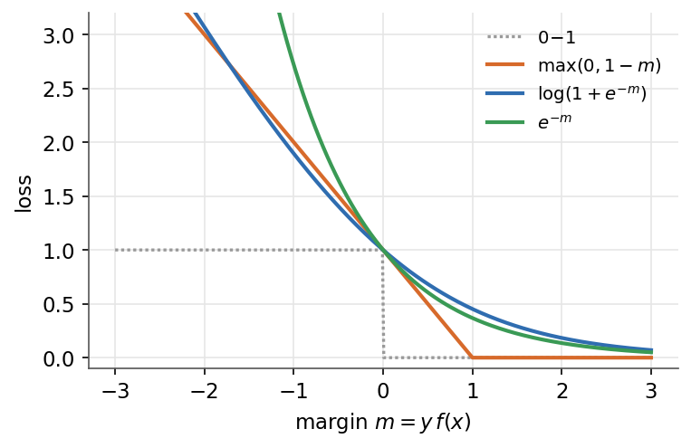 | |
| @@ 38,11 29,11 @@ | |
| ### 2.2.2 Fonction de coût | |
| - | Le coût $J(\theta)$ est défini comme la somme des pertes par exemple sur tout l'ensemble d'entraînement de $m$ exemples : |
| + | Le coût $J(w)$ est défini comme la somme des pertes par exemple sur tout l'ensemble d'entraînement de $m$ exemples : |
| - | $$\boxed{\,J(\theta)=\sum_{i=1}^{m} L\!\left(h_\theta(x^{(i)}),\,y^{(i)}\right)\,}$$ |
| + | $$\boxed{\,J(w)=\sum_{i=1}^{m} L\!\left(h_w(x^{(i)}),\,y^{(i)}\right)\,}$$ |
| - | Entraîner un modèle, c'est choisir $\theta$ qui minimise $J(\theta)$. Les algorithmes qui effectuent cette minimisation (formes fermées, descente de gradient) arrivent avec les modules de modèles. Ce module pose une autre question : que prouve réellement une petite valeur de $J(\theta)$ ? |
| + | Entraîner un modèle, c'est choisir $w$ qui minimise $J(w)$. Les algorithmes qui effectuent cette minimisation (formes fermées, descente de gradient) arrivent avec les modules de modèles. Ce module pose une autre question : que prouve réellement une petite valeur de $J(w)$ ? |
| *Remarque :* le facteur $\tfrac{1}{2}$ de l'erreur quadratique est une convention qui s'annule avec l'exposant lors de la dérivation, laissant un gradient propre. | |
| @@ 50,9 41,9 @@ | |
| Pour rendre tout cela concret, prenons une entrée unique $x$ et ajustons un polynôme de degré $d$ sous la perte quadratique : | |
| - | $$\boxed{ h_\theta(x) = \theta^T \phi(x) = \sum_{j=0}^{d} \theta_j\, x^{j}, \qquad \phi(x) = (1, x, x^2, \dots, x^d) }$$ |
| + | $$\boxed{ h_w(x) = w^T \phi(x) = \sum_{j=0}^{d} w_j\, x^{j}, \qquad \phi(x) = (1, x, x^2, \dots, x^d) }$$ |
| - | Le modèle reste linéaire en $\theta$, les moindres carrés s'appliquent donc tels quels (la forme fermée est dérivée dans [Régression linéaire](/fr/Machine%20Learning/04%20Linear%20regression)). Le degré $d$ n'est pas ajusté avec $\theta$ : il est fixé avant l'ajustement et décide de la flexibilité permise à la courbe. Un tel bouton, choisi plutôt qu'appris, s'appelle un hyperparamètre, et $d$ est notre premier. |
| + | Le modèle reste linéaire en $w$, les moindres carrés s'appliquent donc tels quels (la forme fermée est dérivée dans [Régression linéaire](/fr/Machine%20Learning/04%20Linear%20regression)). Le degré $d$ n'est pas ajusté avec $w$ : il est fixé avant l'ajustement et décide de la flexibilité permise à la courbe. Un tel bouton, choisi plutôt qu'appris, s'appelle un hyperparamètre, et $d$ est notre premier. |
| 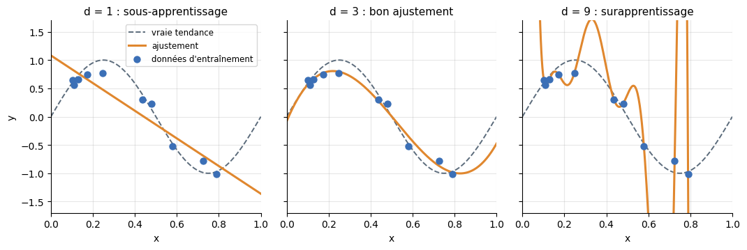 | |
| @@ 84,13 75,13 @@ | |
| ## 2.4 Régularisation | |
| - | Choisir le degré est un réglage grossier : la capacité saute d'entier en entier. Un contrôle plus fin garde une famille flexible mais rend la complexité coûteuse dans le coût lui-même, en ajoutant une pénalité $\Omega(\theta)$ mise à l'échelle par une intensité $\lambda \ge 0$ : |
| + | Choisir le degré est un réglage grossier : la capacité saute d'entier en entier. Un contrôle plus fin garde une famille flexible mais rend la complexité coûteuse dans le coût lui-même, en ajoutant une pénalité $\Omega(w)$ mise à l'échelle par une intensité $\lambda \ge 0$ : |
| - | $$\boxed{\,J_\lambda(\theta)=\sum_{i=1}^{m} L\!\left(h_\theta(x^{(i)}),\,y^{(i)}\right) + \lambda\,\Omega(\theta)\,}$$ |
| + | $$\boxed{\,J_\lambda(w)=\sum_{i=1}^{m} L\!\left(h_w(x^{(i)}),\,y^{(i)}\right) + \lambda\,\Omega(w)\,}$$ |
| - | Le choix classique est la norme au carré $\Omega(\theta) = \lVert \theta \rVert_2^2$, la pénalité ridge. L'ajustement de degré 9 ne se faufile par chaque point qu'à l'aide de coefficients énormes qui se compensent entre les points d'entraînement. La pénalité rend ces coefficients coûteux, le minimiseur échange donc un peu d'erreur d'entraînement contre une courbe bien plus lisse. À $\lambda = 0$ le surapprentissage revient, quand $\lambda \to \infty$ la courbe s'aplatit vers le sous-apprentissage : $\lambda$ parcourt le même cadran biais-variance que le degré, mais continûment. |
| + | Le choix classique est la norme au carré $\Omega(w) = \lVert w \rVert_2^2$, la pénalité ridge. L'ajustement de degré 9 ne se faufile par chaque point qu'à l'aide de coefficients énormes qui se compensent entre les points d'entraînement. La pénalité rend ces coefficients coûteux, le minimiseur échange donc un peu d'erreur d'entraînement contre une courbe bien plus lisse. À $\lambda = 0$ le surapprentissage revient, quand $\lambda \to \infty$ la courbe s'aplatit vers le sous-apprentissage : $\lambda$ parcourt le même cadran biais-variance que le degré, mais continûment. |
| - | *Remarque :* la régularisation ne décide pas de la bonne complexité à votre place, elle convertit un choix discret ($d$) en un choix continu ($\lambda$) plus facile à régler. $\lambda$ est un hyperparamètre comme le degré, choisi par la machinerie de validation de la section suivante. D'où vient la pénalité (un a priori sur $\theta$, via le maximum a posteriori) et ce qu'apporte la variante L1 sont les sujets de [Formulation probabiliste](/fr/Machine%20Learning/03%20Probabilistic%20formulation) et de la [Régression linéaire](/fr/Machine%20Learning/04%20Linear%20regression). |
| + | *Remarque :* la régularisation ne décide pas de la bonne complexité à votre place, elle convertit un choix discret ($d$) en un choix continu ($\lambda$) plus facile à régler. $\lambda$ est un hyperparamètre comme le degré, choisi par la machinerie de validation de la section suivante. D'où vient la pénalité (un a priori sur $w$, via le maximum a posteriori) et ce qu'apporte la variante L1 sont les sujets de [Formulation probabiliste](/fr/Machine%20Learning/03%20Probabilistic%20formulation) et de la [Régression linéaire](/fr/Machine%20Learning/04%20Linear%20regression). |
| ## 2.5 Hyperparamètres, validation et validation croisée | |
| @@ 124,7 115,70 @@ | |
| *Remarque :* choisir le gagnant sur l'ensemble de test gonfle l'estimation. Avec assez de candidats, l'un paraîtra bon par pur hasard, c'est la malédiction du vainqueur, donc sélection et évaluation finale doivent utiliser des données différentes. | |
| - | ## 2.6 Pièges courants de la validation |
| + | ## 2.6 Métriques de régression : de combien se trompe-t-on, en moyenne |
| + | |
| + | La courbe en U de la section 2.3 utilisait déjà une métrique de régression sans la nommer : la RMSE. En régression, la matière première est le résidu $y - \hat{y}$ entre l'étiquette et la prédiction $\hat{y} = h_w(x)$, et les métriques diffèrent par leur façon d'agréger les résidus, ici pour cinq prédictions : |
| + | |
| + | | | $y$ | $\hat{y}$ | $y - \hat{y}$ | |
| + | | --- | --- | --- | --- | |
| + | | exemple 1 | 10 | 12 | $-2$ | |
| + | | exemple 2 | 14 | 13 | $1$ | |
| + | | exemple 3 | 8 | 9 | $-1$ | |
| + | | exemple 4 | 12 | 9 | $3$ | |
| + | | exemple 5 | 16 | 17 | $-1$ | |
| + | |
| + | | Métrique | Formule | Ici | Se lit comme | |
| + | | --- | --- | --- | --- | |
| + | | MSE | $\frac{1}{m}\sum_i \left(y^{(i)} - \hat{y}^{(i)}\right)^2$ | $3{,}2$ | la perte quadratique elle-même, en unités au carré | |
| + | | RMSE | $\sqrt{\text{MSE}}$ | $\approx 1{,}8$ | erreur typique, dans les unités de la cible | |
| + | | MAE | $\frac{1}{m}\sum_i \left\lvert y^{(i)} - \hat{y}^{(i)} \right\rvert$ | $1{,}6$ | écart moyen, robuste aux valeurs aberrantes | |
| + | | $R^2$ | $1 - \sum_i \left(y^{(i)} - \hat{y}^{(i)}\right)^2 \big/ \sum_i \left(y^{(i)} - \bar{y}\right)^2$ | $0{,}6$ | variance expliquée, contre prédire la moyenne | |
| + | |
| + | La moyenne vaut ici $\bar{y} = 12$. La mise au carré rend la MSE et la RMSE quadratiques en chaque résidu, si bien qu'une seule grande erreur les domine, tandis que la MAE ne croît que linéairement : |
| + | |
| + | 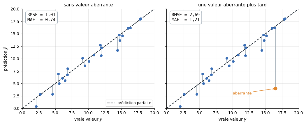 |
| + | |
| + | *Le même ajustement avant et après une seule valeur aberrante : la RMSE triple presque tandis que la MAE bouge bien moins. Que cette sensibilité soit une qualité ou un défaut dépend du coût des grandes erreurs dans l'application.* |
| + | |
| + | *Remarque :* $R^2$ compare le modèle à la base la plus paresseuse, prédire la moyenne $\bar{y}$ pour chaque entrée. $R^2 = 1$ est un ajustement parfait, $R^2 = 0$ ne fait pas mieux que la base, et un $R^2$ négatif, pire que la base, est la façon qu'a la validation de dire que le modèle n'a rien appris. Contrairement à la RMSE et à la MAE, il est sans échelle, il se compare donc entre cibles d'unités différentes. |
| + | |
| + | ## 2.7 Métriques de classification : au-delà d'un simple taux d'erreur |
| + | |
| + | Pour la classification, le chiffre que rapporte la validation n'a pas à être la perte brute. Un classifieur entraîné produit quatre sortes de verdicts : vrais et faux positifs, vrais et faux négatifs. Les compter sur des données mises de côté donne la matrice de confusion, ici pour 29 exemples : |
| + | |
| + | | | prédit $+$ | prédit $-$ | total | |
| + | | --- | --- | --- | --- | |
| + | | réellement $+$ | VP = 11 | FN = 3 | 14 | |
| + | | réellement $-$ | FP = 5 | VN = 10 | 15 | |
| + | |
| + | Chaque métrique phare est un ratio de ces quatre cases : |
| + | |
| + | | Métrique | Formule | Ici | Se lit comme | |
| + | | --- | --- | --- | --- | |
| + | | Justesse (accuracy) | $(VP+VN)/\text{total}$ | $21/29 \approx 0{,}72$ | fraction correcte globale | |
| + | | Rappel (taux de vrais positifs) | $VP/(VP+FN)$ | $11/14 \approx 0{,}79$ | positifs retrouvés | |
| + | | Précision | $VP/(VP+FP)$ | $11/16 \approx 0{,}69$ | positifs signalés qui sont justes | |
| + | | Spécificité | $VN/(VN+FP)$ | $10/15 \approx 0{,}67$ | négatifs préservés | |
| + | | Taux de faux positifs | $FP/(FP+VN)$ | $5/15 \approx 0{,}33$ | négatifs signalés à tort | |
| + | | Score F1 | $2\,\text{Pr}\cdot\text{Re}/(\text{Pr}+\text{Re})$ | $\approx 0{,}73$ | équilibre précision-rappel | |
| + | |
| + | *Remarque :* la justesse seule peut tromper. Avec 1 % de positifs, prédire toujours « négatif » donne 99 % de justesse sans rien trouver. La précision et le rappel comptent les points là où cela compte. |
| + | |
| + | Un classifieur qui produit un score ou une probabilité ne donne pas une matrice de confusion mais une famille : faire glisser le seuil de décision échange des faux positifs contre des faux négatifs. |
| + | |
| + | 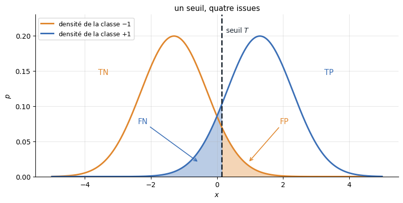 |
| + | |
| + | *Tout ce qui est à droite du seuil est déclaré positif. Pousser le seuil vers la droite réduit les faux positifs (aire orange) mais gonfle les faux négatifs (aire bleue), et inversement.* |
| + | |
| + | Balayer le seuil et tracer le compromis donne la courbe ROC (rappel contre taux de faux positifs, l'idéal est le coin supérieur gauche) et la courbe précision-rappel (l'idéal est le coin supérieur droit). Deux classifieurs se comparent par leurs courbes entières, ou par l'aire sous celles-ci, plutôt que par les chiffres d'un seul seuil. |
| + | |
| + | 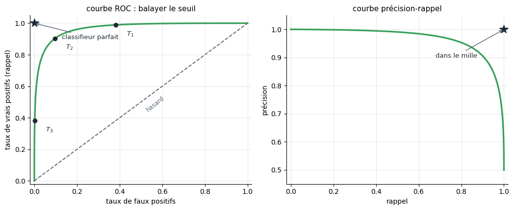 |
| + | |
| + | *Chaque point d'une courbe est un seuil : $T_1$ permissif, $T_3$ strict. Plus la courbe se plie vers son coin idéal, meilleur est le classifieur à tous les compromis.* |
| + | |
| + | *Remarque :* c'est cela, « une métrique adaptée au problème » : on calcule ces métriques sur les blocs de validation ci-dessus pour choisir un modèle, et une seule fois, sur l'ensemble de test, pour le rapporter. |
| + | |
| + | ## 2.8 Pièges courants de la validation |
| Une validation honnête est plus difficile qu'il n'y paraît, et les données réelles brisent souvent les hypothèses habituelles de trois façons. | |
| @@ 140,7 194,7 @@ | |
| *Remarque :* la question honnête derrière toute séparation est toujours la même. Cela aurait-il été connaissable à l'époque, à partir des données dont le modèle disposait réellement ? | |
| - | ## 2.7 La malédiction de la dimensionnalité |
| + | ## 2.9 La malédiction de la dimensionnalité |
| Tout ce qui précède suppose que l'échantillon représente la population au voisinage des points qui comptent. En grande dimension, cette hypothèse se dégrade, et vite. Supposons que les entrées remplissent l'hypercube unité $[0,1]^d$ et que l'on veuille un voisinage autour d'un point qui capture une fraction $r$ des données. Un sous-cube contenant une fraction $r$ du volume doit avoir une arête de longueur : | |
| /dev/null .. fr/Machine Learning/02 General concepts/regression-metrics.png | |
| /dev/null .. fr/Machine Learning/02 General concepts/roc-pr-curves.png | |
| /dev/null .. fr/Machine Learning/02 General concepts/threshold-metrics.png | |
| fr/Machine Learning/03 Probabilistic formulation.md .. | |
| @@ 2,13 2,6 @@ | |
| La probabilité est le langage que le machine learning utilise pour traiter l'incertitude. Ce module énonce les règles pour les variables discrètes et continues, jette un premier regard sur la théorie de l'information, montre la manière bayésienne de transformer des probabilités en décisions, et définit les deux principes d'estimation auxquels le cours revient sans cesse : le maximum de vraisemblance et le maximum a posteriori. | |
| - | **Objectifs** |
| - | - Énoncer les règles de la probabilité pour les variables discrètes et continues. |
| - | - Relier les probabilités conjointe, conditionnelle et marginale par les règles de la somme et du produit et par la règle de Bayes. |
| - | - Mesurer l'incertitude avec l'entropie, l'entropie croisée et la divergence de Kullback-Leibler. |
| - | - Prendre la décision qui minimise la perte espérée, et retrouver le classifieur du maximum a posteriori. |
| - | - Définir les estimateurs du maximum de vraisemblance et du maximum a posteriori. |
| - | |
| ## 3.1 Probabilité, discrète et continue | |
| Une variable aléatoire prend des valeurs avec des probabilités qui sont positives et qui somment ou s'intègrent à un. Une variable discrète a une fonction de masse, une variable continue une densité de probabilité : | |
| @@ 59,21 52,21 @@ | |
| ## 3.5 Maximum de vraisemblance et maximum a posteriori | |
| - | On connaît rarement la vraie distribution, on estime donc ses paramètres $\theta$ à partir des données. Le maximum de vraisemblance choisit le $\theta$ qui rend les données observées les plus probables, maximisé en général comme une somme de log-vraisemblances sur les $m$ exemples : |
| + | On connaît rarement la vraie distribution, on estime donc ses paramètres $w$ à partir des données. Le maximum de vraisemblance choisit le $w$ qui rend les données observées les plus probables, maximisé en général comme une somme de log-vraisemblances sur les $m$ exemples : |
| - | $$\boxed{ \theta_{\mathrm{MV}} = \arg\max_\theta \sum_{i=1}^{m} \log p(x^{(i)} \mid \theta) }$$ |
| + | $$\boxed{ w_{\mathrm{MV}} = \arg\max_w \sum_{i=1}^{m} \log p(x^{(i)} \mid w) }$$ |
| - | En apprentissage supervisé le modèle paramètre la conditionnelle $p(y \mid x; \theta)$, le même principe s'applique donc à la vraisemblance conditionnelle des cibles : |
| + | En apprentissage supervisé le modèle paramètre la conditionnelle $p(y \mid x; w)$, le même principe s'applique donc à la vraisemblance conditionnelle des cibles : |
| - | $$\boxed{ \ell(\theta) = \sum_{i=1}^{m} \log p\!\left(y^{(i)} \mid x^{(i)}; \theta\right) }$$ |
| + | $$\boxed{ \ell(w) = \sum_{i=1}^{m} \log p\!\left(y^{(i)} \mid x^{(i)}; w\right) }$$ |
| - | Maximiser $\ell$ revient à minimiser le coût $J(\theta) = -\ell(\theta)$ : la vue par la vraisemblance et la vue par minimisation du coût de [Concepts généraux](/fr/Machine%20Learning/02%20General%20concepts) sont deux faces d'un même objectif. |
| + | Maximiser $\ell$ revient à minimiser le coût $J(w) = -\ell(w)$ : la vue par la vraisemblance et la vue par minimisation du coût de [Concepts généraux](/fr/Machine%20Learning/02%20General%20concepts) sont deux faces d'un même objectif. |
| - | Le maximum a posteriori maximise plutôt l'a posteriori, qui multiplie la vraisemblance par un a priori sur $\theta$ : |
| + | Le maximum a posteriori maximise plutôt l'a posteriori, qui multiplie la vraisemblance par un a priori sur $w$ : |
| - | $$\boxed{ \theta_{\mathrm{MAP}} = \arg\max_\theta \; p(D \mid \theta)\, p(\theta) }$$ |
| + | $$\boxed{ w_{\mathrm{MAP}} = \arg\max_w \; p(D \mid w)\, p(w) }$$ |
| - | *Remarque :* le maximum a posteriori est le maximum de vraisemblance augmenté d'un a priori. Un a priori gaussien sur $\theta$ devient une pénalité L2 et un a priori de Laplace une pénalité L1, ce qui est exactement la régularisation du module suivant. Avec beaucoup de données l'a priori s'efface et les deux estimateurs coïncident. |
| + | *Remarque :* le maximum a posteriori est le maximum de vraisemblance augmenté d'un a priori. Un a priori gaussien sur $w$ devient une pénalité L2 et un a priori de Laplace une pénalité L1, ce qui est exactement la régularisation du module suivant. Avec beaucoup de données l'a priori s'efface et les deux estimateurs coïncident. |
| *Le module suivant transforme ces principes en un premier modèle concret : la régression linéaire, où maximum de vraisemblance et maximum a posteriori aboutissent tous deux à des ajustements en forme close.* | |
| fr/Machine Learning/04 Linear regression.md .. | |
| @@ 2,21 2,13 @@ | |
| La régression linéaire prédit une cible continue à partir d'un score linéaire. Ce module suit un seul fil de bout en bout : poser le modèle, l'ajuster à des données bruitées par moindres carrés, justifier cet objectif par le maximum de vraisemblance, le régulariser par le maximum a posteriori (ridge, puis son cousin sélectif le lasso), puis élargir le modèle avec les fonctions de base et les prédictions multiples, où les deux mêmes formes closes reviennent inchangées. | |
| - | **Objectifs** |
| - | - Écrire le modèle linéaire et lire sa prédiction comme une droite, un plan ou un hyperplan. |
| - | - Poser le problème d'ajustement sur données bruitées et énoncer l'objectif des moindres carrés. |
| - | - Montrer que le maximum de vraisemblance sous bruit gaussien est exactement les moindres carrés, et dériver l'équation normale. |
| - | - Dériver la régression ridge (weight decay) du maximum a posteriori, en forme close. |
| - | - Opposer les pénalités ridge et lasso : rétrécir ou sélectionner. |
| - | - Généraliser le modèle avec des fonctions de base et aux sorties multiples, en gardant les mêmes formes closes. |
| - | |
| ## 4.1 Le modèle linéaire | |
| L'hypothèse est linéaire en l'entrée augmentée $x \in \mathbb{R}^{n+1}$ avec $x_0 = 1$, la convention de l'[Introduction](/fr/Machine%20Learning/01%20Introduction) : | |
| - | $$\boxed{ h_\theta(x) = \theta^T x = \theta_0 + \theta_1 x_1 + \dots + \theta_n x_n }$$ |
| + | $$\boxed{ h_w(x) = w^T x = w_0 + w_1 x_1 + \dots + w_n x_n }$$ |
| - | $\theta_0$ est le biais (l'ordonnée à l'origine) et les autres coordonnées sont les poids, et replier le biais dans le produit scalaire est exactement ce que la convention $x_0 = 1$ apporte. Géométriquement, la prédiction est une droite pour $n = 1$, un plan pour $n = 2$, un hyperplan au-delà. |
| + | $w_0$ est le biais (l'ordonnée à l'origine) et les autres coordonnées sont les poids, et replier le biais dans le produit scalaire est exactement ce que la convention $x_0 = 1$ apporte. Géométriquement, la prédiction est une droite pour $n = 1$, un plan pour $n = 2$, un hyperplan au-delà. |
| 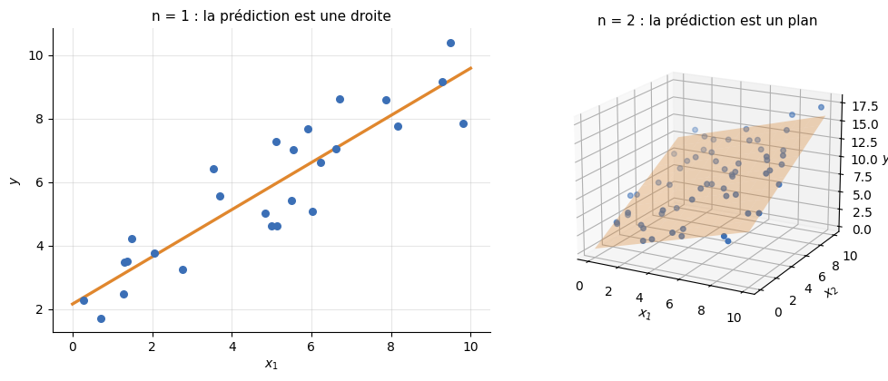 | |
| @@ 24,13 16,13 @@ | |
| ## 4.2 Le problème à résoudre | |
| - | Étant donné l'ensemble d'entraînement $\{(x^{(i)}, y^{(i)})\}_{i=1}^{m}$, on voudrait idéalement $h_\theta(x^{(i)}) = y^{(i)}$ en chaque point. Les cibles réelles sont bruitées (erreurs de mesure, facteurs non modélisés), aucune droite ne passe donc par toutes, et le but devient de commettre la plus petite erreur totale. Les moindres carrés prennent le résidu au carré comme erreur et le somment sur l'ensemble d'entraînement : |
| + | Étant donné l'ensemble d'entraînement $\{(x^{(i)}, y^{(i)})\}_{i=1}^{m}$, on voudrait idéalement $h_w(x^{(i)}) = y^{(i)}$ en chaque point. Les cibles réelles sont bruitées (erreurs de mesure, facteurs non modélisés), aucune droite ne passe donc par toutes, et le but devient de commettre la plus petite erreur totale. Les moindres carrés prennent le résidu au carré comme erreur et le somment sur l'ensemble d'entraînement : |
| - | $$\boxed{ \theta^{*} = \arg\min_\theta \; \sum_{i=1}^{m}\left(\theta^T x^{(i)} - y^{(i)}\right)^2 }$$ |
| + | $$\boxed{ w^{*} = \arg\min_w \; \sum_{i=1}^{m}\left(w^T x^{(i)} - y^{(i)}\right)^2 }$$ |
| 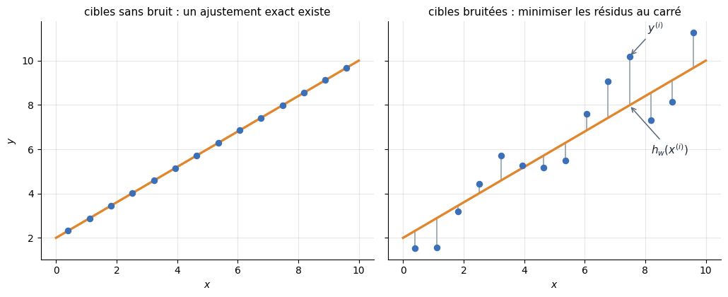 | |
| - | *À gauche : si les cibles étaient sans bruit, le modèle pourrait passer par chaque point. À droite : les cibles réelles se dispersent autour de la tendance, chaque point laisse donc un résidu entre $y^{(i)}$ et la prédiction $h_\theta(x^{(i)})$, et l'ajustement minimise leur somme des carrés (segments gris).* |
| + | *À gauche : si les cibles étaient sans bruit, le modèle pourrait passer par chaque point. À droite : les cibles réelles se dispersent autour de la tendance, chaque point laisse donc un résidu entre $y^{(i)}$ et la prédiction $h_w(x^{(i)})$, et l'ajustement minimise leur somme des carrés (segments gris).* |
| *Remarque :* pourquoi le carré plutôt que, disons, la valeur absolue ? Parce que ce choix est prouvé optimal quand le bruit est gaussien, une question d'entrevue classique que la section suivante décortique. | |
| @@ 38,77 30,125 @@ | |
| Donnons aux données une histoire générative, avec le principe d'estimation de la [Formulation probabiliste](/fr/Machine%20Learning/03%20Probabilistic%20formulation) : chaque cible est la prédiction linéaire plus un bruit gaussien indépendant, | |
| - | $$\boxed{ y^{(i)} = \theta^T x^{(i)} + \varepsilon^{(i)}, \quad \varepsilon^{(i)} \sim \mathcal{N}(0, \sigma^2) }$$ |
| + | $$\boxed{ y^{(i)} = w^T x^{(i)} + \varepsilon^{(i)}, \quad \varepsilon^{(i)} \sim \mathcal{N}(0, \sigma^2) }$$ |
| + | |
| + | donc $p(y^{(i)} \mid x^{(i)}; w) = \mathcal{N}(w^T x^{(i)}, \sigma^2)$. Le maximum de vraisemblance choisit les paramètres sous lesquels les cibles observées sont les plus probables, et il livre deux résultats. D'abord, maximiser la vraisemblance revient exactement à minimiser la somme des erreurs au carré : |
| + | |
| + | $$\boxed{ w_{\mathrm{MV}} = \arg\max_w \; p(y \mid X; w) = \arg\min_w \; \sum_{i=1}^{m}\left(y^{(i)} - w^T x^{(i)}\right)^2 }$$ |
| + | |
| + | Ensuite, le minimiseur a une forme close, l'équation normale, avec $X$ la matrice de conception dont les lignes sont les $x^{(i)T}$ : |
| + | |
| + | $$\boxed{ w_{\mathrm{MV}} = (X^T X)^{-1}X^T y }$$ |
| + | |
| + | une résolution matricielle entre les données et le modèle. |
| + | |
| + | *Remarque :* la première boîte est le fait le plus important du module. Les moindres carrés ne sont pas une convention commode, ils sont l'estimation du maximum de vraisemblance sous bruit gaussien. |
| - | donc $p(y^{(i)} \mid x^{(i)}; \theta) = \mathcal{N}(\theta^T x^{(i)}, \sigma^2)$. La log-vraisemblance des $m$ exemples i.i.d. se sépare en une constante et la somme des carrés : |
| + | <details class="proof"> |
| + | <summary>Preuve : maximiser la vraisemblance, c'est minimiser l'erreur quadratique</summary> |
| - | $$\ell(\theta) = \sum_{i=1}^{m} \log \mathcal{N}\!\left(y^{(i)} \mid \theta^T x^{(i)}, \sigma^2\right) = -\frac{m}{2}\log(2\pi\sigma^2) \;-\; \frac{1}{2\sigma^2}\sum_{i=1}^{m}\left(y^{(i)} - \theta^T x^{(i)}\right)^2$$ |
| + | Les exemples sont i.i.d., la vraisemblance de tout l'ensemble d'entraînement se factorise donc en un produit de densités gaussiennes : |
| - | Ni la constante ni le facteur positif $\tfrac{1}{2\sigma^2}$ ne déplacent l'argmax, donc : |
| + | $$p(y \mid X; w) = \prod_{i=1}^{m} p(y^{(i)} \mid x^{(i)}; w) = \prod_{i=1}^{m} \frac{1}{\sqrt{2\pi\sigma^2}}\, \exp\!\left(-\frac{\left(y^{(i)} - w^T x^{(i)}\right)^2}{2\sigma^2}\right)$$ |
| - | $$\boxed{ \arg\max_\theta \; \ell(\theta) = \arg\min_\theta \; \sum_{i=1}^{m}\left(y^{(i)} - \theta^T x^{(i)}\right)^2 }$$ |
| + | Le logarithme est croissant, il préserve donc l'argmax et transforme le produit en somme, la log-vraisemblance, qui se sépare en une constante et la somme des carrés : |
| - | *Remarque :* cette équivalence est le fait le plus important du module. Les moindres carrés ne sont pas une convention commode, ils sont l'estimation du maximum de vraisemblance sous bruit gaussien. |
| + | $$\ell(w) = \sum_{i=1}^{m} \log \mathcal{N}\!\left(y^{(i)} \mid w^T x^{(i)}, \sigma^2\right) = -\frac{m}{2}\log(2\pi\sigma^2) \;-\; \frac{1}{2\sigma^2}\sum_{i=1}^{m}\left(y^{(i)} - w^T x^{(i)}\right)^2$$ |
| - | Le maximiseur a une forme close. En écrivant l'objectif avec la matrice de conception $X$ et en annulant le gradient, |
| + | Le premier terme ne dépend pas de $w$ et le facteur $\tfrac{1}{2\sigma^2}$ est une constante positive, aucun des deux ne déplace donc l'argmax. Maximiser $\ell$ revient donc à minimiser la somme des erreurs au carré. $\blacksquare$ |
| - | $$\nabla_\theta\, \lVert X\theta - y \rVert^2 = 2\,X^T(X\theta - y) = 0$$ |
| + | </details> |
| - | $$\boxed{ \theta_{\mathrm{MV}} = (X^T X)^{-1}X^T y }$$ |
| + | <details class="proof"> |
| + | <summary>Preuve : l'équation normale</summary> |
| - | l'équation normale, une résolution matricielle entre les données et le modèle. |
| + | Avec la matrice de conception, la somme des carrés est la quadratique $\lVert Xw - y \rVert^2$, une fonction convexe de $w$, son minimum global est donc le point de gradient nul : |
| + | |
| + | $$\nabla_w\, \lVert Xw - y \rVert^2 = 2\,X^T(Xw - y) = 0 \;\Longleftrightarrow\; X^T X\, w = X^T y$$ |
| + | |
| + | Pourvu que $X^T X$ soit inversible (caractéristiques indépendantes, plus d'exemples que de caractéristiques), isoler $w$ donne $w_{\mathrm{MV}} = (X^T X)^{-1}X^T y$. $\blacksquare$ |
| + | |
| + | </details> |
| ## 4.4 Maximum a posteriori : la régression ridge | |
| Le maximum de vraisemblance peut surapprendre, surtout quand le modèle est flexible. L'estimation du maximum a posteriori maximise plutôt l'a posteriori, qui par la règle de Bayes est la vraisemblance multipliée par un a priori sur les paramètres, ici une gaussienne centrée : | |
| - | $$\theta_{\mathrm{MAP}} = \arg\max_\theta \; p(y \mid X, \theta)\, p(\theta), \qquad \theta \sim \mathcal{N}(0, \tau^2 I)$$ |
| + | $$w_{\mathrm{MAP}} = \arg\max_w \; p(y \mid X, w)\, p(w), \qquad w \sim \mathcal{N}(0, \tau^2 I)$$ |
| - | Prendre le logarithme ajoute $-\lVert \theta \rVert^2 / 2\tau^2$ à la log-vraisemblance, et éliminer les constantes laisse des moindres carrés pénalisés : |
| + | Deux résultats à nouveau. L'a priori gaussien se transforme en une pénalité L2 ajoutée aux moindres carrés : |
| - | $$\boxed{ \theta_{\mathrm{MAP}} = \arg\min_\theta \; \sum_{i=1}^{m}\left(y^{(i)} - \theta^T x^{(i)}\right)^2 + \lambda \lVert \theta \rVert_2^2, \quad \lambda = \frac{\sigma^2}{\tau^2} }$$ |
| + | $$\boxed{ w_{\mathrm{MAP}} = \arg\min_w \; \sum_{i=1}^{m}\left(y^{(i)} - w^T x^{(i)}\right)^2 + \lambda \lVert w \rVert_2^2, \quad \lambda = \frac{\sigma^2}{\tau^2} }$$ |
| - | avec, par le même calcul de gradient nul, la forme close : |
| + | et le minimiseur pénalisé garde une forme close : |
| - | $$\boxed{ \theta_{\mathrm{MAP}} = (X^T X + \lambda I)^{-1}X^T y }$$ |
| + | $$\boxed{ w_{\mathrm{MAP}} = (X^T X + \lambda I)^{-1}X^T y }$$ |
| C'est la régression ridge, et la pénalité est souvent appelée weight decay. L'a priori gaussien est devenu la pénalité L2 de [Concepts généraux](/fr/Machine%20Learning/02%20General%20concepts), exactement le lien a priori vers pénalité de la [Formulation probabiliste](/fr/Machine%20Learning/03%20Probabilistic%20formulation). | |
| - | *Remarque :* $\lambda \to 0$ retrouve le maximum de vraisemblance, et un $\lambda$ croissant rétrécit $\theta$ vers zéro et combat le surapprentissage. Un a priori plus fort (petit $\tau$) signifie un $\lambda$ plus grand. Notons aussi que $X^T X + \lambda I$ est toujours inversible pour $\lambda > 0$, ce qui sauve les moindres carrés exactement là où ils s'effondrent : des caractéristiques fortement corrélées, ou plus de caractéristiques que d'exemples. |
| + | *Remarque :* $\lambda \to 0$ retrouve le maximum de vraisemblance, et un $\lambda$ croissant rétrécit $w$ vers zéro et combat le surapprentissage. Un a priori plus fort (petit $\tau$) signifie un $\lambda$ plus grand. Notons aussi que $X^T X + \lambda I$ est toujours inversible pour $\lambda > 0$, ce qui sauve les moindres carrés exactement là où ils s'effondrent : des caractéristiques fortement corrélées, ou plus de caractéristiques que d'exemples. |
| - | ## 4.5 Le lasso : une pénalité qui sélectionne |
| + | <details class="proof"> |
| + | <summary>Preuve : l'a priori gaussien devient la pénalité L2</summary> |
| - | La pénalité ridge venait d'un a priori gaussien. Un a priori de Laplace donne plutôt la pénalité L1, le lien noté dans la [Formulation probabiliste](/fr/Machine%20Learning/03%20Probabilistic%20formulation) : |
| + | Par la règle de Bayes, l'a posteriori est |
| + | |
| + | $$p(w \mid y, X) = \frac{p(y \mid X, w)\, p(w)}{p(y \mid X)}$$ |
| - | $$\boxed{ \theta_{\mathrm{lasso}} = \arg\min_\theta \; \sum_{i=1}^{m}\left(y^{(i)} - \theta^T x^{(i)}\right)^2 + \lambda \lVert \theta \rVert_1 }$$ |
| + | et le dénominateur ne dépend pas de $w$, maximiser l'a posteriori revient donc à maximiser la vraisemblance multipliée par l'a priori. La covariance de l'a priori est généralement inconnue, on la suppose donc isotropique, $\tau^2 I$, ce qui donne la densité |
| - | Le changement paraît minime et sa conséquence est grande : le lasso met certains coefficients exactement à zéro, il sélectionne donc les variables tout en ajustant. Contrairement au ridge il n'a pas de forme close (la pénalité n'est pas dérivable en zéro), il s'ajuste donc par des solveurs convexes. La raison de la sélection est géométrique. La région de contrainte $\lVert \theta \rVert_1 \le t$ est un losange dont les coins sont sur les axes, et les contours elliptiques de l'erreur quadratique tendent à la toucher d'abord en un coin, où une coordonnée est nulle. La boule L2 arrondie n'a pas de coins, le ridge rétrécit donc chaque coefficient doucement sans jamais en annuler un : le ridge stabilise, le lasso sélectionne. |
| + | $$p(w) = \frac{1}{(2\pi\tau^2)^{(n+1)/2}}\, \exp\!\left(-\frac{\lVert w \rVert^2}{2\tau^2}\right)$$ |
| - |  |
| + | En prenant le logarithme et en réutilisant la log-vraisemblance $\ell(w)$ de la preuve précédente, |
| - | *La boule L2 arrondie est touchée hors des axes, gardant chaque coefficient non nul, tandis que le losange L1 est touché en un coin, mettant un coefficient exactement à zéro.* |
| + | $$\log p(y \mid X, w) + \log p(w) = \mathrm{const} \;-\; \frac{1}{2\sigma^2}\sum_{i=1}^{m}\left(y^{(i)} - w^T x^{(i)}\right)^2 \;-\; \frac{1}{2\tau^2}\lVert w \rVert^2$$ |
| - | À mesure que $\lambda$ grandit, davantage de coefficients passent à zéro, traçant le chemin de régularisation du modèle complet jusqu'au modèle vide. |
| + | où la constante rassemble tous les termes indépendants de $w$. Multiplier par $-2\sigma^2$, une constante négative qui change l'argmax en argmin, laisse |
| + | |
| + | $$w_{\mathrm{MAP}} = \arg\min_w \; \sum_{i=1}^{m}\left(y^{(i)} - w^T x^{(i)}\right)^2 + \frac{\sigma^2}{\tau^2}\, \lVert w \rVert^2$$ |
| + | |
| + | et $\lambda = \sigma^2 / \tau^2$ nomme le rapport : plus les données sont bruitées ou plus l'a priori est serré, plus la pénalité est lourde. $\blacksquare$ |
| + | |
| + | </details> |
| + | |
| + | <details class="proof"> |
| + | <summary>Preuve : la forme close du ridge</summary> |
| + | |
| + | Sous forme matricielle, l'objectif est $\lVert Xw - y \rVert^2 + \lambda \lVert w \rVert^2$, toujours une quadratique convexe, la condition de gradient nul trouve donc son minimum global : |
| + | |
| + | $$\nabla_w \left( \lVert Xw - y \rVert^2 + \lambda \lVert w \rVert^2 \right) = 2\,X^T(Xw - y) + 2\lambda w = 0 \;\Longleftrightarrow\; (X^T X + \lambda I)\, w = X^T y$$ |
| + | |
| + | Pour $\lambda > 0$, la matrice $X^T X + \lambda I$ est définie positive, donc inversible, sans condition sur $X$ cette fois : pour tout $v \neq 0$, $v^T (X^T X + \lambda I)\, v = \lVert X v \rVert^2 + \lambda \lVert v \rVert^2 > 0$. Isoler $w$ donne $w_{\mathrm{MAP}} = (X^T X + \lambda I)^{-1} X^T y$. $\blacksquare$ |
| + | |
| + | </details> |
| + | |
| + | ## 4.5 Le lasso : une pénalité qui sélectionne |
| + | |
| + | La pénalité ridge venait d'un a priori gaussien. Un a priori de Laplace donne plutôt la pénalité L1, le lien noté dans la [Formulation probabiliste](/fr/Machine%20Learning/03%20Probabilistic%20formulation) : |
| - |  |
| + | $$\boxed{ w_{\mathrm{lasso}} = \arg\min_w \; \sum_{i=1}^{m}\left(y^{(i)} - w^T x^{(i)}\right)^2 + \lambda \lVert w \rVert_1 }$$ |
| - | *Chaque coefficient rétrécit quand $\lambda$ augmente puis atteint exactement zéro, si bien que le lasso fournit un sous-ensemble compact et interprétable de régresseurs.* |
| + | Le changement paraît minime, ses conséquences non : |
| - | *Remarque :* l'elastic net mêle les deux pénalités, $\lambda\left(\alpha \lVert \theta \rVert_1 + (1-\alpha)\lVert \theta \rVert_2^2\right)$, gardant la sélection du lasso avec la stabilité du ridge face aux caractéristiques corrélées. Comme toujours, $\lambda$ se choisit par la validation croisée de [Concepts généraux](/fr/Machine%20Learning/02%20General%20concepts), en prenant souvent le plus grand $\lambda$ à un écart-type du meilleur pour un modèle plus simple. |
| + | - **Il sélectionne.** Le lasso met certains coefficients exactement à zéro, opérant une sélection de variables tout en ajustant. Le ridge ne fait que rétrécir, sans jamais annuler : le ridge stabilise, le lasso sélectionne. |
| + | - **La raison est géométrique.** La région de contrainte $\lVert w \rVert_1 \le t$ est un losange dont les coins sont sur les axes, et les contours elliptiques de l'erreur quadratique tendent à toucher un coin d'abord, là où une coordonnée est nulle. La boule L2 arrondie n'a pas de coins à accrocher. |
| + | - **$\lambda$ trace un chemin.** Quand $\lambda$ grandit, les coefficients atteignent exactement zéro l'un après l'autre, du modèle complet jusqu'au modèle vide. Comme toujours, $\lambda$ se choisit par la validation croisée de [Concepts généraux](/fr/Machine%20Learning/02%20General%20concepts), souvent le plus grand $\lambda$ à un écart-type du meilleur. |
| + | - **Pas de forme close.** La pénalité L1 n'est pas dérivable en zéro, le lasso s'ajuste donc par des solveurs convexes plutôt que par une formule. |
| + | - **L'elastic net** mêle les deux pénalités, $\lambda\left(\alpha \lVert w \rVert_1 + (1-\alpha)\lVert w \rVert_2^2\right)$, gardant la sélection du lasso avec la stabilité du ridge face aux caractéristiques corrélées. |
| *Remarque :* prédire n'est pas inférer. Sélectionner des variables par lasso puis rapporter les écarts-types des manuels sur les mêmes données est invalide, la malédiction du vainqueur encore : les intervalles ignorent que les données ont déjà choisi les variables. Une inférence honnête demande une division de l'échantillon ou un estimateur débiaisé, la porte d'entrée du machine learning causal. | |
| - | ## 4.6 Fonctions de base : non linéaire en $x$, linéaire en $\theta$ |
| + | ## 4.6 Fonctions de base : non linéaire en $x$, linéaire en $w$ |
| Une droite est souvent trop rigide : le sous-apprentissage de [Concepts généraux](/fr/Machine%20Learning/02%20General%20concepts) apparaissait précisément quand un modèle à faible capacité rencontrait une tendance courbe. La solution n'est pas d'abandonner la machinerie linéaire mais de projeter l'entrée dans un espace plus grand, là où la relation est linéaire : | |
| - | $$\boxed{ h_\theta(x) = \theta^T \phi(x) = \sum_{j=0}^{M-1} \theta_j\, \phi_j(x), \qquad \phi_0(x) = 1 }$$ |
| + | $$\boxed{ h_w(x) = w^T \phi(x) = \sum_{j=0}^{M-1} w_j\, \phi_j(x), \qquad \phi_0(x) = 1 }$$ |
| - | Les $\phi_j$ sont des fonctions de base, fixées avant l'entraînement. Avec $\phi(x) = (1, x, x^2, \dots, x^d)$ elles donnent la régression polynomiale, l'exemple fil rouge de [Concepts généraux](/fr/Machine%20Learning/02%20General%20concepts), et l'identité $\phi(x) = x$ retrouve tout ce qui précède. Le modèle peut désormais être follement non linéaire en $x$ tout en restant linéaire en $\theta$, rien ne change donc dans l'ajustement : on empile les $\phi(x^{(i)})^T$ comme lignes de la matrice de conception $\Phi \in \mathbb{R}^{m \times M}$ et les deux formes closes reviennent telles quelles : |
| + | Les $\phi_j$ sont des fonctions de base, fixées avant l'entraînement. Avec $\phi(x) = (1, x, x^2, \dots, x^d)$ elles donnent la régression polynomiale, l'exemple fil rouge de [Concepts généraux](/fr/Machine%20Learning/02%20General%20concepts), et l'identité $\phi(x) = x$ retrouve tout ce qui précède. Le modèle peut désormais être follement non linéaire en $x$ tout en restant linéaire en $w$, rien ne change donc dans l'ajustement : on empile les $\phi(x^{(i)})^T$ comme lignes de la matrice de conception $\Phi \in \mathbb{R}^{m \times M}$ et les deux formes closes reviennent telles quelles : |
| - | $$\boxed{ \theta_{\mathrm{MV}} = (\Phi^T \Phi)^{-1}\Phi^T y, \qquad \theta_{\mathrm{MAP}} = (\Phi^T \Phi + \lambda I)^{-1}\Phi^T y }$$ |
| + | $$\boxed{ w_{\mathrm{MV}} = (\Phi^T \Phi)^{-1}\Phi^T y, \qquad w_{\mathrm{MAP}} = (\Phi^T \Phi + \lambda I)^{-1}\Phi^T y }$$ |
| - | *Remarque :* la base (sa famille et sa taille $M$) est un hyperparamètre, choisi avant l'entraînement, tandis que $\theta$ est appris. Choisir $M$ et $\lambda$ est le problème de sélection de modèle réglé par la validation croisée de [Concepts généraux](/fr/Machine%20Learning/02%20General%20concepts). |
| + | *Remarque :* la base (sa famille et sa taille $M$) est un hyperparamètre, choisi avant l'entraînement, tandis que $w$ est appris. Choisir $M$ et $\lambda$ est le problème de sélection de modèle réglé par la validation croisée de [Concepts généraux](/fr/Machine%20Learning/02%20General%20concepts). |
| ## 4.7 Prédictions multiples | |
| @@ 126,10 166,10 @@ | |
| | | Formule | | |
| | --- | --- | | |
| - | | Modèle | $h_\theta(x) = \theta^T \phi(x)$ | |
| - | | Maximum de vraisemblance (moindres carrés) | $\theta_{\mathrm{MV}} = (\Phi^T \Phi)^{-1}\Phi^T y$ | |
| - | | Maximum a posteriori (ridge) | $\theta_{\mathrm{MAP}} = (\Phi^T \Phi + \lambda I)^{-1}\Phi^T y$ | |
| - | | Paramètres, appris | $\theta$ (ou $W$ pour $K$ sorties) | |
| + | | Modèle | $h_w(x) = w^T \phi(x)$ | |
| + | | Maximum de vraisemblance (moindres carrés) | $w_{\mathrm{MV}} = (\Phi^T \Phi)^{-1}\Phi^T y$ | |
| + | | Maximum a posteriori (ridge) | $w_{\mathrm{MAP}} = (\Phi^T \Phi + \lambda I)^{-1}\Phi^T y$ | |
| + | | Paramètres, appris | $w$ (ou $W$ pour $K$ sorties) | |
| | Hyperparamètres, choisis par validation | la base $\phi$ et sa taille $M$, la pénalité $\lambda$ | | |
| *Le même score linéaire, passé dans une fonction de compression au lieu d'être lu directement, transforme la régression en classification, le sujet du module suivant.* | |
| fr/Machine Learning/04 Linear regression/ideal-vs-noisy.png .. | |
| fr/Machine Learning/04 Linear regression/l1-l2-geometry.png .. /dev/null | |
| fr/Machine Learning/04 Linear regression/regularization-path.png .. /dev/null | |
| fr/Machine Learning/05 Linear classification.md .. | |
| @@ 1,43 1,26 @@ | |
| # 5. Classification linéaire | |
| - | La classification prédit une étiquette discrète à partir du même score linéaire $\theta^T x$. Ce module passe en revue les classifieurs linéaires classiques comme un seul menu : les moindres carrés, qui supposent des classes de forme gaussienne et admettent une forme close, et le perceptron et la régression logistique, qui ne supposent rien sur la distribution et s'ajustent par descente de gradient. La régularisation ferme le module. |
| - | |
| - | **Objectifs** |
| - | - Lire un classifieur linéaire comme un hyperplan séparateur dont le score donne le côté, rendant la prédiction aussi rapide qu'un produit scalaire. |
| - | - Situer les méthodes classiques selon leur hypothèse (gaussienne ou aucune) et leur ajustement (forme close ou descente de gradient). |
| - | - Classer par moindres carrés, en binaire et en multiclasse, et voir où cela casse. |
| - | - Entraîner le perceptron à partir de son critère, et connaître sa garantie de convergence et ses limites. |
| - | - Distinguer la descente de gradient par lots de la stochastique, et savoir que des optimiseurs plus élaborés existent. |
| - | - Ajuster la régression logistique par descente de gradient sur l'entropie croisée, en binaire et en multiclasse. |
| - | - Régulariser n'importe lequel de ces ajustements avec une pénalité, la vue maximum a posteriori. |
| + | La classification prédit une étiquette discrète à partir du même score linéaire $w^T x$. Ce module passe en revue les classifieurs linéaires classiques comme un seul menu : les moindres carrés, qui supposent des classes de forme gaussienne et admettent une forme close, et le perceptron et la régression logistique, qui ne supposent rien sur la distribution et s'ajustent par descente de gradient. La régularisation ferme le module. |
| ## 5.1 Le séparateur linéaire | |
| Un classifieur linéaire attribue la classe d'après le signe du score linéaire, et l'ensemble des entrées de score nul est la frontière de décision : | |
| - | $$\boxed{ h_\theta(x) = \mathrm{sign}(\theta^T x), \qquad \theta^T x = 0 \ \text{est la frontière} }$$ |
| - | |
| - | La frontière est un hyperplan : une droite avec deux caractéristiques, un plan avec trois. Le signe du score dit de quel côté de l'hyperplan l'entrée tombe, et sa grandeur à quelle distance de la frontière elle se trouve. Avec $\theta = (-4, 1, 2)$ (biais en tête, sur l'entrée augmentée), le point $x = (3, 2)$ obtient $-4 + 3 + 4 = 3$ et tombe devant l'hyperplan, tandis que $x = (1, 1)$ obtient $-4 + 1 + 2 = -1$ et tombe derrière. |
| - | |
| - | *Remarque :* deux avantages pratiques en découlent. Une fois l'entraînement terminé, l'ensemble d'entraînement peut être jeté, et prédire coûte un seul produit scalaire. |
| + | $$\boxed{ h_w(x) = \mathrm{sign}(w^T x), \qquad w^T x = 0 \ \text{est la frontière} }$$ |
| - | ## 5.2 Un menu de méthodes |
| + | La frontière est un hyperplan : une droite avec deux caractéristiques, un plan avec trois. Le signe du score dit de quel côté de l'hyperplan l'entrée tombe, et sa grandeur à quelle distance de la frontière elle se trouve. Avec $w = (-4, 1, 2)$ (biais en tête, sur l'entrée augmentée), le point $x = (3, 2)$ obtient $-4 + 3 + 4 = 3$ et tombe devant l'hyperplan, tandis que $x = (1, 1)$ obtient $-4 + 1 + 2 = -1$ et tombe derrière. |
| - | Les méthodes classiques ajustent cet hyperplan, et elles se séparent nettement selon ce qu'elles supposent des données et la façon dont elles se résolvent. |
| + | 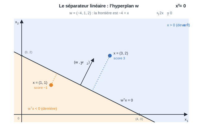 |
| - | | Méthode | Hypothèse sur les données | Ajustement | |
| - | | --- | --- | --- | |
| - | | Moindres carrés | classes de forme gaussienne | forme close (inversion de matrice) | |
| - | | Perceptron | aucune | descente de gradient | |
| - | | Régression logistique | aucune | descente de gradient | |
| + | *L'hyperplan $w^T x = 0$ coupe l'espace d'entrée en deux : avec $w = (-4, 1, 2)$ la frontière est la droite $-4 + x_1 + 2x_2 = 0$, normale à $(w_1, w_2)$. Le point $(3, 2)$ obtient $3$ et tombe devant, $(1, 1)$ obtient $-1$ et tombe derrière, et la grandeur du score croît avec la distance à la frontière (pointillés).* |
| - | Les moindres carrés héritent du confort de la forme close de la [Régression linéaire](/fr/Machine%20Learning/04%20Linear%20regression) et le paient d'une hypothèse de distribution. Les deux autres ne supposent rien et le paient d'une optimisation itérative. |
| + | *Remarque :* deux avantages pratiques en découlent. Une fois l'entraînement terminé, l'ensemble d'entraînement peut être jeté, et prédire coûte un seul produit scalaire. |
| - | ## 5.3 Les moindres carrés comme classifieur |
| + | ## 5.2 Les moindres carrés comme classifieur |
| Codons les deux classes $y \in \{-1, +1\}$, traitons-les comme des cibles de régression, et tout le module [Régression linéaire](/fr/Machine%20Learning/04%20Linear%20regression) s'applique tel quel, forme close comprise : | |
| - | $$\boxed{ \theta = (X^T X)^{-1}X^T y, \qquad h_\theta(x) = \mathrm{sign}(\theta^T x) }$$ |
| + | $$\boxed{ w = (X^T X)^{-1}X^T y, \qquad h_w(x) = \mathrm{sign}(w^T x) }$$ |
| Pour $K > 2$ classes, on code chaque étiquette comme une ligne one-hot de $Y \in \mathbb{R}^{m \times K}$ et on réutilise les prédictions multiples de la [Régression linéaire](/fr/Machine%20Learning/04%20Linear%20regression), en prédisant la classe au score le plus élevé : | |
| @@ 49,25 32,31 @@ | |
| *Sans points extrêmes, moindres carrés et régression logistique concordent. Ajouter des points lointains et pourtant bien classés fait basculer la frontière des moindres carrés dans l'erreur, tandis que la régression logistique bouge à peine.* | |
| - | ## 5.4 Le perceptron |
| + | ## 5.3 Le perceptron |
| - | ### 5.4.1 Modèle, perte et mise à jour |
| + | ### 5.3.1 Le modèle : un neurone |
| La première méthode sans hypothèse prend la définition du classifieur linéaire au pied de la lettre, un produit scalaire suivi d'une activation dure, le neurone historique : | |
| - | $$\boxed{ h_\theta(x) = \mathrm{sign}(\theta^T x), \qquad y \in \{-1, +1\} }$$ |
| + | $$\boxed{ h_w(x) = \mathrm{sign}(w^T x), \qquad y \in \{-1, +1\} }$$ |
| 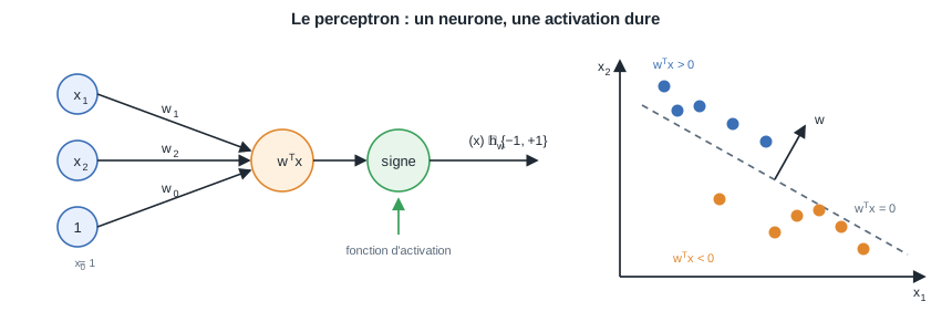 | |
| - | *À gauche : le perceptron est un seul neurone, les entrées pondérées sommées dans le score $\theta^T x$ puis passées dans une activation signe dure. À droite : ce signe coupe l'espace d'entrée le long de l'hyperplan $\theta^T x = 0$.* |
| + | *À gauche : le perceptron est un seul neurone, les entrées pondérées sommées dans le score $w^T x$ puis passées dans une activation signe dure. À droite : ce signe coupe l'espace d'entrée le long de l'hyperplan $w^T x = 0$.* |
| - | L'ajustement demande une perte, et compter les erreurs ne fonctionne pas : le compte est constant par morceaux, son gradient est donc nul presque partout. Le critère du perceptron pénalise plutôt chaque point mal classé selon la distance à laquelle il se trouve du mauvais côté. Une erreur signifie $y^{(i)}\,\theta^T x^{(i)} < 0$, donc sur l'ensemble $\mathcal{M}$ des points mal classés : |
| + | ### 5.3.2 La fonction de perte : le critère du perceptron |
| - | $$\boxed{ E(\theta) = -\sum_{i \in \mathcal{M}} y^{(i)}\, \theta^T x^{(i)} }$$ |
| + | L'ajustement demande une perte, et compter les erreurs ne fonctionne pas : le compte est constant par morceaux, son gradient est donc nul presque partout. Le critère du perceptron pénalise plutôt chaque point mal classé selon la distance à laquelle il se trouve du mauvais côté. Une erreur signifie $y^{(i)}\,w^T x^{(i)} < 0$, donc sur l'ensemble $\mathcal{M}$ des points mal classés : |
| - | toujours positif et linéaire par morceaux. Le minimiser introduit l'outil de base de tout ce qui, dans ce cours, n'a pas de forme close, la descente de gradient : avancer les paramètres à répétition à l'opposé du gradient de la perte, mis à l'échelle par un taux d'apprentissage $\alpha > 0$ : |
| + | $$\boxed{ E(w) = -\sum_{i \in \mathcal{M}} y^{(i)}\, w^T x^{(i)} }$$ |
| - | $$\boxed{\,\theta \leftarrow \theta - \alpha\,\nabla_\theta E(\theta)\,}$$ |
| + | toujours positif et linéaire par morceaux. |
| + | |
| + | ### 5.3.3 Optimisation : la descente de gradient |
| + | |
| + | Minimiser le critère introduit l'outil de base de tout ce qui, dans ce cours, n'a pas de forme close, la descente de gradient : avancer les paramètres à répétition à l'opposé du gradient de la perte, mis à l'échelle par un taux d'apprentissage $\alpha > 0$ : |
| + | |
| + | $$\boxed{\,w \leftarrow w - \alpha\,\nabla_w E(w)\,}$$ |
| La variante par lots calcule le gradient sur tout l'ensemble d'entraînement avant chaque pas, une descente lisse qui relit chaque exemple à chaque fois. La variante stochastique (SGD) avance sur un exemple à la fois, peu coûteuse et bruitée, et c'est le choix par défaut sur les grands jeux de données. Si $\alpha$ est trop grand les itérés peuvent diverger, s'il est trop petit la convergence se traîne. | |
| @@ 75,21 64,21 @@ | |
| Sur un seul exemple mal classé le gradient du critère vaut $-y^{(i)} x^{(i)}$, le pas stochastique est donc la mise à jour du perceptron : sur une erreur, | |
| - | $$\boxed{ \theta \leftarrow \theta + \alpha\, y^{(i)} x^{(i)} }$$ |
| + | $$\boxed{ w \leftarrow w + \alpha\, y^{(i)} x^{(i)} }$$ |
| - | et aucune mise à jour sinon. Dans le codage $\{0, 1\}$ c'est la mise à jour résidu fois l'entrée $\theta_j \leftarrow \theta_j + \alpha\,(y^{(i)} - h_\theta(x^{(i)}))\,x_j^{(i)}$. |
| + | et aucune mise à jour sinon. Dans le codage $\{0, 1\}$ c'est la mise à jour résidu fois l'entrée $w_j \leftarrow w_j + \alpha\,(y^{(i)} - h_w(x^{(i)}))\,x_j^{(i)}$. |
| 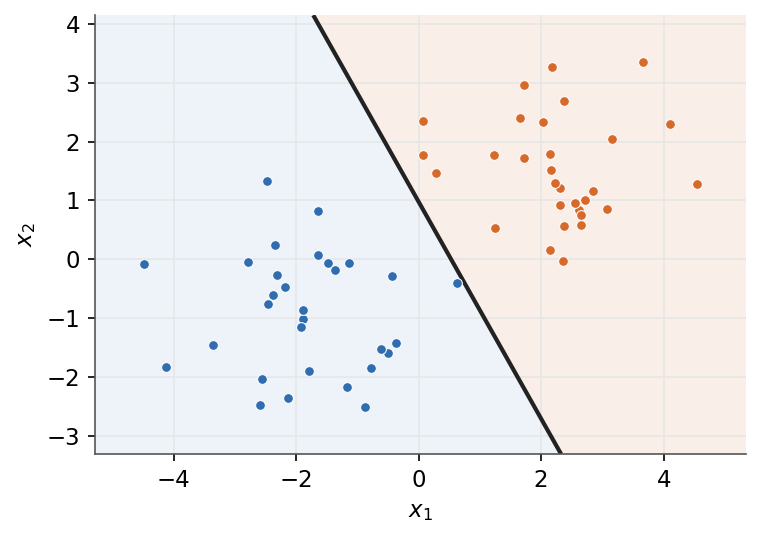 | |
| *Le perceptron trouve un hyperplan séparateur, pas nécessairement celui de marge maximale que la machine à vecteurs de support choisira.* | |
| - | ### 5.4.2 Perceptron multiclasse |
| + | ### 5.3.4 Perceptron multiclasse |
| - | Avec $k$ classes, on garde un vecteur de poids $\theta_c$ par classe et on prédit celle au plus fort score. Sur une erreur, on récompense la vraie classe et on pénalise la classe prédite : |
| + | Avec $k$ classes, on garde un vecteur de poids $w_c$ par classe et on prédit celle au plus fort score. Sur une erreur, on récompense la vraie classe et on pénalise la classe prédite : |
| - | $$\boxed{ \hat{y} = \arg\max_c \theta_c^T x, \qquad \theta_{y} \mathrel{+}= \alpha x, \quad \theta_{\hat{y}} \mathrel{-}= \alpha x }$$ |
| + | $$\boxed{ \hat{y} = \arg\max_c w_c^T x, \qquad w_{y} \mathrel{+}= \alpha x, \quad w_{\hat{y}} \mathrel{-}= \alpha x }$$ |
| - | La vue en réseau s'étend naturellement : un neurone de score par classe, et un argmax là où le perceptron binaire avait un signe. En rassemblant les $\theta_c$ comme colonnes d'une matrice $W \in \mathbb{R}^{(n+1) \times k}$, un seul produit $W^T x$ calcule tous les scores à la fois, et les scores découpent l'espace d'entrée en $k$ régions, chacune revendiquée par la classe au score le plus élevé. |
| + | La vue en réseau s'étend naturellement : un neurone de score par classe, et un argmax là où le perceptron binaire avait un signe. En rassemblant les $w_c$ comme colonnes d'une matrice $W \in \mathbb{R}^{(n+1) \times k}$, un seul produit $W^T x$ calcule tous les scores à la fois, et les scores découpent l'espace d'entrée en $k$ régions, chacune revendiquée par la classe au score le plus élevé. |
| 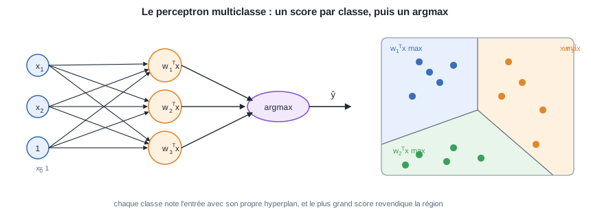 | |
| @@ 99,87 88,165 @@ | |
| $$ W^T x = \begin{bmatrix} -2 & -4 & 1 \\ -4 & 2 & 4 \\ -6 & 4 & -5 \end{bmatrix}\begin{bmatrix} 1 \\ 1{,}1 \\ -2{,}0 \end{bmatrix} = \begin{bmatrix} -8{,}4 \\ -9{,}8 \\ 8{,}4 \end{bmatrix} $$ | |
| - | Le troisième score l'emporte, l'entrée est donc affectée à la classe 3. En lisant la troisième ligne, ce score vaut $\theta_3^T x = -6 + 4 \times 1{,}1 + (-5) \times (-2{,}0) = 8{,}4$. |
| + | Le troisième score l'emporte, l'entrée est donc affectée à la classe 3. En lisant la troisième ligne, ce score vaut $w_3^T x = -6 + 4 \times 1{,}1 + (-5) \times (-2{,}0) = 8{,}4$. |
| - | ### 5.4.3 Convergence et limites |
| + | ### 5.3.5 Convergence et limites |
| Si les données sont linéairement séparables, le perceptron converge en un nombre fini de mises à jour, sinon les poids oscillent indéfiniment. Et comme le critère vaut zéro sur tout hyperplan séparateur, tous comptent comme « optimaux », y compris ceux qui frôlent les données. | |
| *Remarque :* trois améliorations corrigent ces limites, et chacune ouvre un module. Une activation et une perte lisses donnent la régression logistique, section suivante. Les marges et les fonctions de base mènent à la [machine à vecteurs de support](/fr/Machine%20Learning/07%20Support%20Vector%20Machines). Empiler les neurones en couches donne les [réseaux de neurones multi-couches](/fr/Machine%20Learning/06%20Multilayer%20neural%20networks), point de départ du cours de Deep Learning. | |
| - | ## 5.5 La régression logistique |
| + | ## 5.4 La régression logistique |
| - | ### 5.5.1 Une activation lisse |
| + | ### 5.4.1 Le modèle : une activation lisse |
| - | La régression logistique garde le neurone mais remplace l'échelon dur par la sigmoïde lisse, si bien que la sortie est la probabilité de la classe positive ($y \in \{0, 1\}$) : |
| + | La régression logistique garde le neurone mais remplace l'échelon dur par la sigmoïde lisse, si bien que la sortie est la probabilité de la classe positive ($y \in \{0, 1\}$). On la note toujours $\hat{y}$, mais l'estimation de l'étiquette est désormais douce : le $\hat{y}$ du perceptron était une classe dure, celui de la régression logistique est une probabilité, et le seuiller à $\tfrac{1}{2}$ redonne une classe quand il en faut une : |
| - | $$\boxed{ \phi = p(y = 1 \mid x; \theta) = \sigma(\theta^T x) = \frac{1}{1 + e^{-\theta^T x}} }$$ |
| + | $$\boxed{ \hat{y} = p(y = 1 \mid x; w) = \sigma(w^T x) = \frac{1}{1 + e^{-w^T x}} }$$ |
| 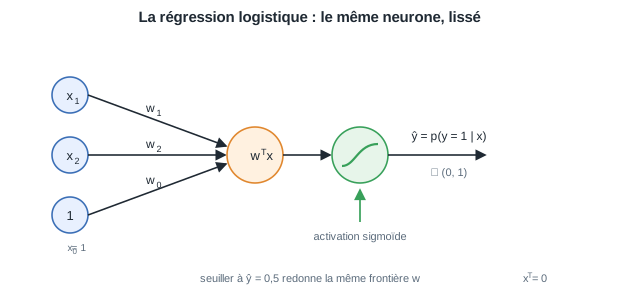 | |
| - | *Le même neurone avec l'échelon remplacé par la sigmoïde : la sortie devient la probabilité $\phi = p(y = 1 \mid x)$, et la seuiller à $\tfrac{1}{2}$ redonne la même frontière $\theta^T x = 0$.* |
| + | *Le même neurone avec l'échelon remplacé par la sigmoïde : la sortie devient la probabilité $\hat{y} = p(y = 1 \mid x)$, et la seuiller à $\tfrac{1}{2}$ redonne la même frontière $w^T x = 0$.* |
| *Remarque :* la sigmoïde n'est pas un choix de compression arbitraire. Écrire l'a posteriori avec la règle de Bayes donne $p(C_1 \mid x) = 1/(1 + e^{-a})$ avec $a = \ln \frac{p(x \mid C_1)\,p(C_1)}{p(x \mid C_0)\,p(C_0)}$, donc une sortie logistique bien entraînée est exactement une probabilité a posteriori. | |
| - | ### 5.5.2 L'entropie croisée et son gradient |
| + | ### 5.4.2 La fonction de perte : l'entropie croisée |
| La vraisemblance d'étiquettes de Bernoulli, passée au $-\log$, donne la perte d'entropie croisée : | |
| - | $$\boxed{ L(\theta) = -\sum_{i=1}^{m}\left[ y^{(i)}\log \phi^{(i)} + (1 - y^{(i)})\log(1 - \phi^{(i)}) \right] }$$ |
| + | $$\boxed{ L(w) = -\sum_{i=1}^{m}\left[ y^{(i)}\log \hat{y}^{(i)} + (1 - y^{(i)})\log(1 - \hat{y}^{(i)}) \right] }$$ |
| + | |
| + | <details class="proof"> |
| + | <summary>Preuve : le maximum de vraisemblance donne l'entropie croisée</summary> |
| + | |
| + | Le modèle dit que chaque étiquette est un tirage de Bernoulli de probabilité de succès $\hat{y}^{(i)} = \sigma(w^T x^{(i)})$, et les deux cas se replient en une seule expression : |
| + | |
| + | $$p(y^{(i)} \mid x^{(i)}; w) = \left(\hat{y}^{(i)}\right)^{y^{(i)}}\left(1 - \hat{y}^{(i)}\right)^{1 - y^{(i)}}$$ |
| + | |
| + | puisque $y^{(i)} \in \{0, 1\}$ sélectionne le facteur : l'expression vaut $\hat{y}^{(i)}$ quand $y^{(i)} = 1$ et $1 - \hat{y}^{(i)}$ quand $y^{(i)} = 0$. Les exemples sont i.i.d., la vraisemblance de l'ensemble d'entraînement se factorise donc, comme dans la [Régression linéaire](/fr/Machine%20Learning/04%20Linear%20regression) : |
| + | |
| + | $$p(y \mid X; w) = \prod_{i=1}^{m} \left(\hat{y}^{(i)}\right)^{y^{(i)}}\left(1 - \hat{y}^{(i)}\right)^{1 - y^{(i)}}$$ |
| + | |
| + | Le logarithme préserve l'argmax, transforme le produit en somme et fait descendre les exposants : |
| + | |
| + | $$\ell(w) = \sum_{i=1}^{m}\left[ y^{(i)}\log \hat{y}^{(i)} + (1 - y^{(i)})\log(1 - \hat{y}^{(i)}) \right]$$ |
| + | |
| + | Maximiser $\ell$ revient à minimiser $-\ell$, qui est exactement $L(w)$. L'entropie croisée est l'opposé de la log-vraisemblance de Bernoulli, le même principe d'estimation qui faisait des moindres carrés la réponse sous bruit gaussien. $\blacksquare$ |
| + | |
| + | </details> |
| + | |
| + | ### 5.4.3 Optimisation : la descente de gradient |
| Contrairement aux moindres carrés, cette perte n'a pas de minimiseur en forme close : la sigmoïde rend les équations de stationnarité transcendantes, l'ajustement revient donc à la même descente de gradient que le perceptron. Dériver l'entropie croisée à travers la sigmoïde récompense l'effort : presque tout se simplifie et le gradient se réduit au résidu fois l'entrée : | |
| - | $$\boxed{ \theta_j \leftarrow \theta_j - \alpha \sum_{i=1}^{m}\left(\phi^{(i)} - y^{(i)}\right)x_j^{(i)} }$$ |
| + | $$\boxed{ w_j \leftarrow w_j - \alpha \sum_{i=1}^{m}\left(\hat{y}^{(i)} - y^{(i)}\right)x_j^{(i)} }$$ |
| + | |
| + | <details class="proof"> |
| + | <summary>Preuve : le gradient se réduit au résidu fois l'entrée</summary> |
| + | |
| + | Notons le score $z^{(i)} = w^T x^{(i)}$, de sorte que $\hat{y}^{(i)} = \sigma(z^{(i)})$. La dérivation repose sur une seule identité, la sigmoïde qui se dérive en elle-même : |
| - | *Remarque :* contrairement au perceptron, le gradient fait intervenir chaque point d'entraînement, pas seulement les mal classés : chaque point tire proportionnellement à son résidu $\phi^{(i)} - y^{(i)}$. C'est ce qui rend la régression logistique plus stable que le perceptron et utilisable sur des données non séparables. |
| + | $$\sigma'(z) = \frac{e^{-z}}{\left(1 + e^{-z}\right)^2} = \frac{1}{1 + e^{-z}} \cdot \frac{e^{-z}}{1 + e^{-z}} = \sigma(z)\left(1 - \sigma(z)\right)$$ |
| + | |
| + | puisque $\tfrac{e^{-z}}{1 + e^{-z}} = 1 - \sigma(z)$. Prenons maintenant la perte d'un seul exemple, $L^{(i)} = -\left[y^{(i)}\log \hat{y}^{(i)} + (1 - y^{(i)})\log(1 - \hat{y}^{(i)})\right]$, et suivons la règle de dérivation en chaîne à travers ses trois étages, de la perte à la sortie, de la sortie au score, du score au poids : |
| + | |
| + | $$\frac{\partial L^{(i)}}{\partial \hat{y}^{(i)}} = -\frac{y^{(i)}}{\hat{y}^{(i)}} + \frac{1 - y^{(i)}}{1 - \hat{y}^{(i)}} = \frac{\hat{y}^{(i)} - y^{(i)}}{\hat{y}^{(i)}\left(1 - \hat{y}^{(i)}\right)}, \qquad \frac{\partial \hat{y}^{(i)}}{\partial z^{(i)}} = \hat{y}^{(i)}\left(1 - \hat{y}^{(i)}\right), \qquad \frac{\partial z^{(i)}}{\partial w_j} = x_j^{(i)}$$ |
| + | |
| + | (la première égalité met les deux fractions au dénominateur commun $\hat{y}^{(i)}(1 - \hat{y}^{(i)})$, et la deuxième est l'identité de la sigmoïde ci-dessus). En multipliant les trois, le dénominateur du premier facteur est exactement le deuxième facteur, et tout se simplifie : |
| + | |
| + | $$\frac{\partial L^{(i)}}{\partial w_j} = \frac{\hat{y}^{(i)} - y^{(i)}}{\hat{y}^{(i)}\left(1 - \hat{y}^{(i)}\right)} \cdot \hat{y}^{(i)}\left(1 - \hat{y}^{(i)}\right) \cdot x_j^{(i)} = \left(\hat{y}^{(i)} - y^{(i)}\right) x_j^{(i)}$$ |
| + | |
| + | Sommer sur l'ensemble d'entraînement donne $\partial L / \partial w_j = \sum_{i=1}^{m} (\hat{y}^{(i)} - y^{(i)})\, x_j^{(i)}$, et brancher ce gradient dans la règle de descente $w \leftarrow w - \alpha\, \nabla_w L$ est la mise à jour encadrée. $\blacksquare$ |
| + | |
| + | </details> |
| + | |
| + | *Remarque :* contrairement au perceptron, le gradient fait intervenir chaque point d'entraînement, pas seulement les mal classés : chaque point tire proportionnellement à son résidu $\hat{y}^{(i)} - y^{(i)}$. C'est ce qui rend la régression logistique plus stable que le perceptron et utilisable sur des données non séparables. |
| 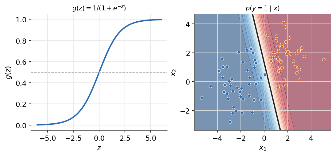 | |
| *À gauche : la sigmoïde envoie tout score dans l'intervalle (0, 1). À droite : la frontière de décision et la probabilité prédite.* | |
| - | ### 5.5.3 Multiclasse : la softmax |
| + | ### 5.4.4 Multiclasse : la softmax |
| + | |
| + | Pour $k$ classes, la sigmoïde se généralise en la softmax : un vecteur de poids $w_c$, donc un score, par classe, des exponentielles qui rendent les scores positifs, et une normalisation qui en fait une distribution. En notant $\hat{y}_c$ la probabilité prédite de la classe $c$, comme $\hat{y}$ était la probabilité de la classe positive ci-dessus : |
| + | |
| + | $$\boxed{ \hat{y}_c = p(y = c \mid x; w) = \frac{\exp(w_c^T x)}{\sum_{j=1}^{k}\exp(w_j^T x)} }$$ |
| - | Pour $k$ classes, la sigmoïde se généralise en la softmax, un vecteur de poids par classe, normalisé en une distribution : |
| + | 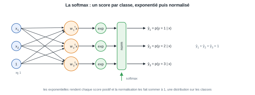 |
| - | $$\boxed{ p(y = c \mid x; \theta) = \frac{\exp(\theta_c^T x)}{\sum_{j=1}^{k}\exp(\theta_j^T x)} }$$ |
| + | *Le réseau multiclasse à tête softmax : chaque classe note l'entrée, les exponentielles rendent les scores positifs, et la normalisation les transforme en probabilités de somme 1. C'est le réseau du perceptron multiclasse avec l'argmax remplacé par une tête lisse et dérivable.* |
| Avec des étiquettes one-hot, la perte est l'entropie croisée catégorielle $L = -\sum_i \log p(y^{(i)} \mid x^{(i)})$, dont le gradient garde la même forme résidu fois l'entrée. | |
| | | sigmoïde | softmax | | |
| | --- | --- | --- | | |
| | classes | 2 | $k$ | | |
| - | | sortie | une probabilité $\phi$ | une distribution sur $k$ classes | |
| + | | sortie | une probabilité $\hat{y}$ | une distribution sur $k$ classes | |
| | relation | la softmax à $k = 2$ se réduit à la sigmoïde | généralise la sigmoïde | | |
| - | ## 5.6 La classification régularisée |
| + | <details class="proof"> |
| + | <summary>Preuve : la softmax à k = 2 est la sigmoïde</summary> |
| + | |
| + | Avec deux classes, la softmax note l'entrée deux fois, $w_1$ pour la classe positive et $w_0$ pour la classe négative : |
| + | |
| + | $$p(y = 1 \mid x; w) = \frac{e^{w_1^T x}}{e^{w_1^T x} + e^{w_0^T x}}$$ |
| - | Rien ne fixe l'échelle de $\theta$ : le doubler ne déplace aucune frontière du perceptron et ne fait qu'affûter les probabilités de la régression logistique, et des vecteurs de poids différents peuvent produire des scores identiques. La recette du maximum a posteriori de la [Régression linéaire](/fr/Machine%20Learning/04%20Linear%20regression) s'applique telle quelle, en ajoutant une pénalité à la perte minimisée, quelle qu'elle soit : |
| + | Diviser le numérateur et le dénominateur par $e^{w_1^T x}$ laisse |
| - | $$\boxed{ J_\lambda(\theta) = \sum_{i=1}^{m} L\!\left(h_\theta(x^{(i)}),\,y^{(i)}\right) + \lambda\,\Omega(\theta), \qquad \Omega(\theta) = \lVert \theta \rVert_2^2 \ \text{ou} \ \lVert \theta \rVert_1 }$$ |
| + | $$p(y = 1 \mid x; w) = \frac{1}{1 + e^{-(w_1 - w_0)^T x}} = \sigma\!\left((w_1 - w_0)^T x\right)$$ |
| - | Pour l'entropie croisée avec la pénalité L2, le gradient gagne simplement une traction vers zéro, $\sum_i (\phi^{(i)} - y^{(i)})\,x^{(i)} + 2\lambda\theta$. |
| + | la sigmoïde appliquée à la différence des scores. Seule la différence $w = w_1 - w_0$ compte (le fait général derrière cela : décaler chaque $w_c$ du même vecteur laisse la softmax inchangée), un seul vecteur de poids suffit donc, exactement le modèle binaire par lequel cette section a commencé. Lue dans l'autre sens, c'est la recette de la généralisation : donner à chaque classe son propre score $w_c^T x$, exponentier pour rendre les scores positifs, normaliser pour qu'ils somment à un, et le cas à deux classes se replie en une seule sigmoïde. $\blacksquare$ |
| + | |
| + | </details> |
| + | |
| + | ## 5.5 La classification régularisée |
| + | |
| + | Rien ne fixe l'échelle de $w$ : le doubler ne déplace aucune frontière du perceptron et ne fait qu'affûter les probabilités de la régression logistique, et des vecteurs de poids différents peuvent produire des scores identiques. La recette du maximum a posteriori de la [Régression linéaire](/fr/Machine%20Learning/04%20Linear%20regression) s'applique telle quelle, en ajoutant une pénalité à la perte minimisée, quelle qu'elle soit : |
| + | |
| + | $$\boxed{ J_\lambda(w) = \sum_{i=1}^{m} L\!\left(h_w(x^{(i)}),\,y^{(i)}\right) + \lambda\,\Omega(w), \qquad \Omega(w) = \lVert w \rVert_2^2 \ \text{ou} \ \lVert w \rVert_1 }$$ |
| + | |
| + | Pour l'entropie croisée avec la pénalité L2, le gradient gagne simplement une traction vers zéro, $\sum_i (\hat{y}^{(i)} - y^{(i)})\,x^{(i)} + 2\lambda w$. |
| *Remarque :* les bibliothèques exposent exactement ce menu, une perte plus une pénalité (le `SGDClassifier` de scikit-learn prend un argument `loss` et un argument `penalty`). L'intensité $\lambda$ se choisit par la validation de [Concepts généraux](/fr/Machine%20Learning/02%20General%20concepts), et le comportement sélectif du lasso est couvert dans la [Régression linéaire](/fr/Machine%20Learning/04%20Linear%20regression). | |
| - | ## 5.7 Résumé |
| + | ## 5.6 Résumé |
| - | Les méthodes sans hypothèse partagent une seule mise à jour, le résidu fois l'entrée : |
| + | Les méthodes classiques ajustent toutes le même hyperplan, et elles se séparent nettement selon ce qu'elles supposent des données et la façon dont elles se résolvent : les moindres carrés héritent du confort de la forme close de la [Régression linéaire](/fr/Machine%20Learning/04%20Linear%20regression) et le paient d'une hypothèse de distribution, le perceptron et la régression logistique ne supposent rien et le paient d'une optimisation itérative. Algorithme par algorithme, les formules qui définissent chacun : |
| - | | Modèle | Activation | Mise à jour (un exemple) | |
| - | | --- | --- | --- | |
| - | | Perceptron | échelon | $\theta_j \leftarrow \theta_j + \alpha\,(y - h_\theta(x))\,x_j$ (erreurs seulement) | |
| - | | Régression linéaire | identité | $\theta_j \leftarrow \theta_j + \alpha\,(y - \theta^T x)\,x_j$ | |
| - | | Régression logistique | sigmoïde ou softmax | $\theta_j \leftarrow \theta_j + \alpha\,(y - \phi)\,x_j$ | |
| + | **Les moindres carrés**, la méthode avec hypothèse et forme close : |
| - | *Remarque :* seule l'activation diffère (échelon, identité, sigmoïde ou softmax). Le cours de Deep Learning reprend précisément ce fil, en empilant de telles unités en couches. |
| + | | | Formule | |
| + | | --- | --- | |
| + | | Hypothèse sur les données | classes de forme gaussienne | |
| + | | Activation | identité pour entraîner (régression sur des cibles $\pm 1$), puis $\mathrm{sign}(w^T x)$ pour prédire | |
| + | | Perte | erreur quadratique $\sum_{i=1}^{m}\left(w^T x^{(i)} - y^{(i)}\right)^2$ | |
| + | | Ajustement | forme close $w = (X^T X)^{-1}X^T y$, aucune itération | |
| + | | Multiclasse | lignes one-hot de $Y$, $W = (X^T X)^{-1}X^T Y$, prédire $\arg\max_k\,(W^T x)_k$ | |
| - | Et les pertes en un coup d'œil : |
| + | **Le perceptron**, guidé par les erreurs et sans hypothèse : |
| - | | Perte | Pénalise | Utilisée par | |
| - | | --- | --- | --- | |
| - | | Critère du perceptron | les points mal classés seulement | perceptron | |
| - | | Charnière $\max(0,\,1 - y\,\theta^T x)$ | les erreurs et les petites marges | [SVM](/fr/Machine%20Learning/07%20Support%20Vector%20Machines) | |
| - | | Entropie croisée | chaque point, selon son résidu | régression logistique | |
| + | | | Formule | |
| + | | --- | --- | |
| + | | Hypothèse sur les données | aucune | |
| + | | Activation | échelon, $h_w(x) = \mathrm{sign}(w^T x)$, $y \in \{-1, +1\}$ | |
| + | | Perte | critère du perceptron $E(w) = -\sum_{i \in \mathcal{M}} y^{(i)}\, w^T x^{(i)}$, points mal classés seulement | |
| + | | Gradient | $\nabla_w E = -\sum_{i \in \mathcal{M}} y^{(i)} x^{(i)}$ | |
| + | | Mise à jour | $w \leftarrow w + \alpha\, y^{(i)} x^{(i)}$ sur une erreur, rien sinon | |
| + | | Multiclasse | $\hat{y} = \arg\max_c\, w_c^T x$, puis $w_{y} \mathrel{+}= \alpha x$ et $w_{\hat{y}} \mathrel{-}= \alpha x$ | |
| + | | Convergence | finie si les données sont séparables, oscille sinon | |
| + | |
| + | **La régression logistique**, probabiliste et sans hypothèse : |
| + | |
| + | | | Formule | |
| + | | --- | --- | |
| + | | Hypothèse sur les données | aucune | |
| + | | Activation | sigmoïde, $\hat{y} = \sigma(w^T x) = \tfrac{1}{1 + e^{-w^T x}}$, une probabilité, $y \in \{0, 1\}$ | |
| + | | Perte | entropie croisée $L(w) = -\sum_{i=1}^{m}\left[ y^{(i)}\log \hat{y}^{(i)} + (1 - y^{(i)})\log(1 - \hat{y}^{(i)}) \right]$ | |
| + | | Gradient | $\nabla_{w_j} L = \sum_{i=1}^{m}\left(\hat{y}^{(i)} - y^{(i)}\right)x_j^{(i)}$, chaque point tire selon son résidu | |
| + | | Mise à jour | $w_j \leftarrow w_j - \alpha \sum_{i=1}^{m}\left(\hat{y}^{(i)} - y^{(i)}\right)x_j^{(i)}$ | |
| + | | Multiclasse | softmax $\hat{y}_c = \tfrac{\exp(w_c^T x)}{\sum_{j}\exp(w_j^T x)}$ et l'entropie croisée catégorielle | |
| + | |
| + | *Remarque :* lues côte à côte, la mise à jour du perceptron (dans son codage $\{0, 1\}$) et celle de la régression logistique sont la même formule, le résidu fois l'entrée, et seule l'activation change (l'échelon pour le perceptron, la sigmoïde pour la régression logistique, et l'identité de la régression linéaire complète la famille). Le cours de Deep Learning reprend précisément ce fil, en empilant de telles unités en couches. Une perte manque volontairement à ce menu, la charnière $\max(0,\,1 - y\,w^T x)$, qui pénalise les petites marges autant que les erreurs : elle appartient à la [SVM](/fr/Machine%20Learning/07%20Support%20Vector%20Machines). |
| *Les modèles linéaires étant couverts, le module suivant empile ces briques en réseaux de neurones multi-couches.* | |
| /dev/null .. fr/Machine Learning/05 Linear classification/hyperplane.svg | |
| @@ 0,0 1,41 @@ | |
| + | <svg xmlns="http://www.w3.org/2000/svg" viewBox="0 0 640 430" width="640" height="430" font-family="Helvetica, Arial, sans-serif"> |
| + | <defs> |
| + | <marker id="arrow" viewBox="0 0 10 10" refX="8.5" refY="5" markerWidth="7" markerHeight="7" orient="auto-start-reverse"><path d="M0 0L10 5L0 10z" fill="#1f2933"/></marker> |
| + | </defs> |
| + | <rect width="640" height="430" fill="#ffffff"/> |
| + | <text x="320" y="24" font-size="15" font-weight="600" fill="#1f2933" text-anchor="middle">Le séparateur linéaire : l'hyperplan w<tspan dy="-4" font-size="10">T</tspan><tspan dy="4">x = 0</tspan></text> |
| + | <text x="320" y="46" font-size="12" fill="#5b6b7b" text-anchor="middle">w = (−4, 1, 2) : la frontière est −4 + x<tspan dy="3" font-size="9">1</tspan><tspan dy="-3"> + 2x</tspan><tspan dy="3" font-size="9">2</tspan><tspan dy="-3"> = 0</tspan></text> |
| + | |
| + | <polygon points="45,167.5 500,395 610,395 610,60 45,60" fill="#e8f0fe"/> |
| + | <polygon points="45,167.5 500,395 45,395" fill="#fff1e0"/> |
| + | |
| + | <line x1="45" y1="370" x2="605" y2="370" stroke="#1f2933" stroke-width="1.7" marker-end="url(#arrow)"/> |
| + | <line x1="70" y1="395" x2="70" y2="65" stroke="#1f2933" stroke-width="1.7" marker-end="url(#arrow)"/> |
| + | <text x="600" y="390" font-size="12" fill="#1f2933" text-anchor="middle">x<tspan dy="4" font-size="9">1</tspan></text> |
| + | <text x="52" y="75" font-size="12" fill="#1f2933" text-anchor="middle">x<tspan dy="4" font-size="9">2</tspan></text> |
| + | <text x="60" y="386" font-size="10" fill="#5b6b7b" text-anchor="middle">0</text> |
| + | |
| + | <line x1="45" y1="167.5" x2="500" y2="395" stroke="#1f2933" stroke-width="2"/> |
| + | <text x="390" y="328" font-size="12" fill="#1f2933" text-anchor="start">w<tspan dy="-4" font-size="8">T</tspan><tspan dy="4">x = 0</tspan></text> |
| + | |
| + | <line x1="66" y1="180" x2="74" y2="180" stroke="#1f2933" stroke-width="1.4"/> |
| + | <text x="80" y="172" font-size="10" fill="#5b6b7b" text-anchor="start">(0, 2)</text> |
| + | <line x1="450" y1="366" x2="450" y2="374" stroke="#1f2933" stroke-width="1.4"/> |
| + | <text x="450" y="388" font-size="10" fill="#5b6b7b" text-anchor="middle">(4, 0)</text> |
| + | |
| + | <line x1="260" y1="275" x2="302.8" y2="189.5" stroke="#1f2933" stroke-width="1.7" marker-end="url(#arrow)"/> |
| + | <text x="252" y="205" font-size="12" fill="#1f2933" text-anchor="end">(w<tspan dy="4" font-size="9">1</tspan><tspan dy="-4">, w</tspan><tspan dy="4" font-size="9">2</tspan><tspan dy="-4">)</tspan></text> |
| + | |
| + | <text x="600" y="85" font-size="12" fill="#3b6fb6" text-anchor="end">w<tspan dy="-4" font-size="8">T</tspan><tspan dy="4">x > 0 (devant)</tspan></text> |
| + | <text x="90" y="355" font-size="12" fill="#e0872e" text-anchor="start">w<tspan dy="-4" font-size="8">T</tspan><tspan dy="4">x < 0 (derrière)</tspan></text> |
| + | |
| + | <line x1="355" y1="180" x2="298" y2="294" stroke="#3b6fb6" stroke-width="1.4" stroke-dasharray="3 4"/> |
| + | <circle cx="355" cy="180" r="6" fill="#3b6fb6"/> |
| + | <text x="367" y="176" font-size="12" fill="#1f2933" text-anchor="start">x = (3, 2)</text> |
| + | <text x="367" y="192" font-size="11" fill="#3b6fb6" text-anchor="start">score 3</text> |
| + | |
| + | <line x1="165" y1="275" x2="184" y2="237" stroke="#e0872e" stroke-width="1.4" stroke-dasharray="3 4"/> |
| + | <circle cx="165" cy="275" r="6" fill="#e0872e"/> |
| + | <text x="153" y="271" font-size="12" fill="#1f2933" text-anchor="end">x = (1, 1)</text> |
| + | <text x="153" y="287" font-size="11" fill="#e0872e" text-anchor="end">score −1</text> |
| + | </svg> |
| fr/Machine Learning/05 Linear classification/logistic-neuron.svg .. | |
| @@ 17,12 17,12 @@ | |
| <line x1="88" y1="95" x2="226" y2="146" stroke="#1f2933" stroke-width="1.6" marker-end="url(#arrow)"/> | |
| <line x1="88" y1="155" x2="225" y2="155" stroke="#1f2933" stroke-width="1.6" marker-end="url(#arrow)"/> | |
| <line x1="88" y1="215" x2="226" y2="164" stroke="#1f2933" stroke-width="1.6" marker-end="url(#arrow)"/> | |
| - | <text x="150" y="112" font-size="12" fill="#1f2933" text-anchor="middle">θ<tspan dy="4" font-size="9">1</tspan></text> |
| - | <text x="150" y="148" font-size="12" fill="#1f2933" text-anchor="middle">θ<tspan dy="4" font-size="9">2</tspan></text> |
| - | <text x="150" y="184" font-size="12" fill="#1f2933" text-anchor="middle">θ<tspan dy="4" font-size="9">0</tspan></text> |
| + | <text x="150" y="112" font-size="12" fill="#1f2933" text-anchor="middle">w<tspan dy="4" font-size="9">1</tspan></text> |
| + | <text x="150" y="148" font-size="12" fill="#1f2933" text-anchor="middle">w<tspan dy="4" font-size="9">2</tspan></text> |
| + | <text x="150" y="184" font-size="12" fill="#1f2933" text-anchor="middle">w<tspan dy="4" font-size="9">0</tspan></text> |
| <circle cx="255" cy="155" r="28" fill="#fff1e0" stroke="#e0872e" stroke-width="1.6"/> | |
| - | <text x="255" y="160" font-size="13" fill="#1f2933" text-anchor="middle">θ<tspan dy="-5" font-size="9">T</tspan><tspan dy="5" font-size="13">x</tspan></text> |
| + | <text x="255" y="160" font-size="13" fill="#1f2933" text-anchor="middle">w<tspan dy="-5" font-size="9">T</tspan><tspan dy="5" font-size="13">x</tspan></text> |
| <line x1="283" y1="155" x2="330" y2="155" stroke="#1f2933" stroke-width="1.6" marker-end="url(#arrow)"/> | |
| @@ 30,11 30,11 @@ | |
| <path d="M342 166 C 355 166, 358 144, 378 144" fill="none" stroke="#38a05a" stroke-width="2.2"/> | |
| <line x1="388" y1="155" x2="485" y2="155" stroke="#1f2933" stroke-width="1.6" marker-end="url(#arrow)"/> | |
| - | <text x="449" y="140" font-size="12" fill="#1f2933" text-anchor="middle">φ = p(y = 1 | x)</text> |
| + | <text x="449" y="140" font-size="12" fill="#1f2933" text-anchor="middle">ŷ = p(y = 1 | x)</text> |
| <text x="449" y="176" font-size="11" fill="#5b6b7b" text-anchor="middle">∈ (0, 1)</text> | |
| <line x1="360" y1="222" x2="360" y2="190" stroke="#38a05a" stroke-width="1.7" marker-end="url(#arrowgreen)"/> | |
| <text x="360" y="240" font-size="11" fill="#5b6b7b" text-anchor="middle">activation sigmoïde</text> | |
| - | <text x="310" y="282" font-size="11" fill="#5b6b7b" text-anchor="middle">seuiller à φ = 0,5 redonne la même frontière θ<tspan dy="-4" font-size="8">T</tspan><tspan dy="4">x = 0</tspan></text> |
| + | <text x="310" y="282" font-size="11" fill="#5b6b7b" text-anchor="middle">seuiller à ŷ = 0,5 redonne la même frontière w<tspan dy="-4" font-size="8">T</tspan><tspan dy="4">x = 0</tspan></text> |
| </svg> | |
| fr/Machine Learning/05 Linear classification/multiclass-neuron.svg .. | |
| @@ 24,11 24,11 @@ | |
| <line x1="71" y1="215" x2="214" y2="215" stroke="#1f2933" stroke-width="1.1" marker-end="url(#arrow)"/> | |
| <circle cx="240" cy="95" r="24" fill="#fff1e0" stroke="#e0872e" stroke-width="1.6"/> | |
| - | <text x="240" y="100" font-size="12" fill="#1f2933" text-anchor="middle">θ<tspan dy="4" font-size="8">1</tspan><tspan dy="-10" font-size="8">T</tspan><tspan dy="6" font-size="12">x</tspan></text> |
| + | <text x="240" y="100" font-size="12" fill="#1f2933" text-anchor="middle">w<tspan dy="4" font-size="8">1</tspan><tspan dy="-10" font-size="8">T</tspan><tspan dy="6" font-size="12">x</tspan></text> |
| <circle cx="240" cy="155" r="24" fill="#fff1e0" stroke="#e0872e" stroke-width="1.6"/> | |
| - | <text x="240" y="160" font-size="12" fill="#1f2933" text-anchor="middle">θ<tspan dy="4" font-size="8">2</tspan><tspan dy="-10" font-size="8">T</tspan><tspan dy="6" font-size="12">x</tspan></text> |
| + | <text x="240" y="160" font-size="12" fill="#1f2933" text-anchor="middle">w<tspan dy="4" font-size="8">2</tspan><tspan dy="-10" font-size="8">T</tspan><tspan dy="6" font-size="12">x</tspan></text> |
| <circle cx="240" cy="215" r="24" fill="#fff1e0" stroke="#e0872e" stroke-width="1.6"/> | |
| - | <text x="240" y="220" font-size="12" fill="#1f2933" text-anchor="middle">θ<tspan dy="4" font-size="8">3</tspan><tspan dy="-10" font-size="8">T</tspan><tspan dy="6" font-size="12">x</tspan></text> |
| + | <text x="240" y="220" font-size="12" fill="#1f2933" text-anchor="middle">w<tspan dy="4" font-size="8">3</tspan><tspan dy="-10" font-size="8">T</tspan><tspan dy="6" font-size="12">x</tspan></text> |
| <ellipse cx="405" cy="155" rx="45" ry="22" fill="#f2e9fd" stroke="#8257d6" stroke-width="1.6"/> | |
| <text x="405" y="160" font-size="12" fill="#1f2933" text-anchor="middle">argmax</text> | |
| @@ 63,9 63,9 @@ | |
| <circle cx="780" cy="210" r="5" fill="#e0872e"/> | |
| <circle cx="730" cy="140" r="5" fill="#e0872e"/> | |
| - | <text x="568" y="74" font-size="11" fill="#3b6fb6" text-anchor="start">θ<tspan dy="3" font-size="8">1</tspan><tspan dy="-7" font-size="8">T</tspan><tspan dy="4" font-size="11">x max</tspan></text> |
| - | <text x="572" y="223" font-size="11" fill="#38a05a" text-anchor="start">θ<tspan dy="3" font-size="8">2</tspan><tspan dy="-7" font-size="8">T</tspan><tspan dy="4" font-size="11">x max</tspan></text> |
| - | <text x="828" y="74" font-size="11" fill="#e0872e" text-anchor="end">θ<tspan dy="3" font-size="8">3</tspan><tspan dy="-7" font-size="8">T</tspan><tspan dy="4" font-size="11">x max</tspan></text> |
| + | <text x="568" y="74" font-size="11" fill="#3b6fb6" text-anchor="start">w<tspan dy="3" font-size="8">1</tspan><tspan dy="-7" font-size="8">T</tspan><tspan dy="4" font-size="11">x max</tspan></text> |
| + | <text x="572" y="223" font-size="11" fill="#38a05a" text-anchor="start">w<tspan dy="3" font-size="8">2</tspan><tspan dy="-7" font-size="8">T</tspan><tspan dy="4" font-size="11">x max</tspan></text> |
| + | <text x="828" y="74" font-size="11" fill="#e0872e" text-anchor="end">w<tspan dy="3" font-size="8">3</tspan><tspan dy="-7" font-size="8">T</tspan><tspan dy="4" font-size="11">x max</tspan></text> |
| <text x="405" y="300" font-size="11" fill="#5b6b7b" text-anchor="middle">chaque classe note l'entrée avec son propre hyperplan, et le plus grand score revendique la région</text> | |
| </svg> | |
| fr/Machine Learning/05 Linear classification/perceptron-neuron.svg .. | |
| @@ 17,12 17,12 @@ | |
| <line x1="88" y1="85" x2="226" y2="136" stroke="#1f2933" stroke-width="1.6" marker-end="url(#arrow)"/> | |
| <line x1="88" y1="145" x2="225" y2="145" stroke="#1f2933" stroke-width="1.6" marker-end="url(#arrow)"/> | |
| <line x1="88" y1="205" x2="226" y2="154" stroke="#1f2933" stroke-width="1.6" marker-end="url(#arrow)"/> | |
| - | <text x="150" y="102" font-size="12" fill="#1f2933" text-anchor="middle">θ<tspan dy="4" font-size="9">1</tspan></text> |
| - | <text x="150" y="138" font-size="12" fill="#1f2933" text-anchor="middle">θ<tspan dy="4" font-size="9">2</tspan></text> |
| - | <text x="150" y="174" font-size="12" fill="#1f2933" text-anchor="middle">θ<tspan dy="4" font-size="9">0</tspan></text> |
| + | <text x="150" y="102" font-size="12" fill="#1f2933" text-anchor="middle">w<tspan dy="4" font-size="9">1</tspan></text> |
| + | <text x="150" y="138" font-size="12" fill="#1f2933" text-anchor="middle">w<tspan dy="4" font-size="9">2</tspan></text> |
| + | <text x="150" y="174" font-size="12" fill="#1f2933" text-anchor="middle">w<tspan dy="4" font-size="9">0</tspan></text> |
| <circle cx="255" cy="145" r="28" fill="#fff1e0" stroke="#e0872e" stroke-width="1.6"/> | |
| - | <text x="255" y="150" font-size="13" fill="#1f2933" text-anchor="middle">θ<tspan dy="-5" font-size="9">T</tspan><tspan dy="5" font-size="13">x</tspan></text> |
| + | <text x="255" y="150" font-size="13" fill="#1f2933" text-anchor="middle">w<tspan dy="-5" font-size="9">T</tspan><tspan dy="5" font-size="13">x</tspan></text> |
| <line x1="283" y1="145" x2="330" y2="145" stroke="#1f2933" stroke-width="1.6" marker-end="url(#arrow)"/> | |
| @@ 30,7 30,7 @@ | |
| <text x="360" y="150" font-size="13" fill="#1f2933" text-anchor="middle">signe</text> | |
| <line x1="388" y1="145" x2="485" y2="145" stroke="#1f2933" stroke-width="1.6" marker-end="url(#arrow)"/> | |
| - | <text x="445" y="131" font-size="12" fill="#1f2933" text-anchor="middle">h<tspan dy="4" font-size="9">θ</tspan><tspan dy="-4">(x) ∈ {−1, +1}</tspan></text> |
| + | <text x="445" y="131" font-size="12" fill="#1f2933" text-anchor="middle">h<tspan dy="4" font-size="9">w</tspan><tspan dy="-4">(x) ∈ {−1, +1}</tspan></text> |
| <line x1="360" y1="212" x2="360" y2="180" stroke="#38a05a" stroke-width="1.7" marker-end="url(#arrowgreen)"/> | |
| <text x="360" y="230" font-size="11" fill="#5b6b7b" text-anchor="middle">fonction d'activation</text> | |
| @@ 41,17 41,17 @@ | |
| <text x="543" y="64" font-size="12" fill="#1f2933" text-anchor="middle">x<tspan dy="4" font-size="9">2</tspan></text> | |
| <line x1="580" y1="95" x2="820" y2="230" stroke="#5b6b7b" stroke-width="1.7" stroke-dasharray="6 5"/> | |
| - | <text x="772" y="192" font-size="11" fill="#5b6b7b" text-anchor="start">θ<tspan dy="-4" font-size="8">T</tspan><tspan dy="4">x = 0</tspan></text> |
| + | <text x="772" y="192" font-size="11" fill="#5b6b7b" text-anchor="start">w<tspan dy="-4" font-size="8">T</tspan><tspan dy="4">x = 0</tspan></text> |
| <line x1="700" y1="162" x2="727" y2="114" stroke="#1f2933" stroke-width="1.7" marker-end="url(#arrow)"/> | |
| - | <text x="736" y="112" font-size="12" fill="#1f2933" text-anchor="start">θ</text> |
| + | <text x="736" y="112" font-size="12" fill="#1f2933" text-anchor="start">w</text> |
| <circle cx="600" cy="78" r="5.5" fill="#3b6fb6"/> | |
| <circle cx="632" cy="96" r="5.5" fill="#3b6fb6"/> | |
| <circle cx="662" cy="112" r="5.5" fill="#3b6fb6"/> | |
| <circle cx="692" cy="128" r="5.5" fill="#3b6fb6"/> | |
| <circle cx="612" cy="100" r="5.5" fill="#3b6fb6"/> | |
| - | <text x="590" y="62" font-size="11" fill="#3b6fb6" text-anchor="start">θ<tspan dy="-4" font-size="8">T</tspan><tspan dy="4">x > 0</tspan></text> |
| + | <text x="590" y="62" font-size="11" fill="#3b6fb6" text-anchor="start">w<tspan dy="-4" font-size="8">T</tspan><tspan dy="4">x > 0</tspan></text> |
| <circle cx="650" cy="180" r="5.5" fill="#e0872e"/> | |
| <circle cx="700" cy="210" r="5.5" fill="#e0872e"/> | |
| @@ 59,5 59,5 @@ | |
| <circle cx="780" cy="225" r="5.5" fill="#e0872e"/> | |
| <circle cx="720" cy="195" r="5.5" fill="#e0872e"/> | |
| <circle cx="760" cy="205" r="5.5" fill="#e0872e"/> | |
| - | <text x="608" y="237" font-size="11" fill="#e0872e" text-anchor="start">θ<tspan dy="-4" font-size="8">T</tspan><tspan dy="4">x < 0</tspan></text> |
| + | <text x="608" y="237" font-size="11" fill="#e0872e" text-anchor="start">w<tspan dy="-4" font-size="8">T</tspan><tspan dy="4">x < 0</tspan></text> |
| </svg> | |
| /dev/null .. fr/Machine Learning/05 Linear classification/softmax-neuron.svg | |
| @@ 0,0 1,65 @@ | |
| + | <svg xmlns="http://www.w3.org/2000/svg" viewBox="0 0 860 320" width="860" height="320" font-family="Helvetica, Arial, sans-serif"> |
| + | <defs> |
| + | <marker id="arrow" viewBox="0 0 10 10" refX="8.5" refY="5" markerWidth="6" markerHeight="6" orient="auto-start-reverse"><path d="M0 0L10 5L0 10z" fill="#1f2933"/></marker> |
| + | <marker id="arrowgreen" viewBox="0 0 10 10" refX="8.5" refY="5" markerWidth="7" markerHeight="7" orient="auto-start-reverse"><path d="M0 0L10 5L0 10z" fill="#38a05a"/></marker> |
| + | </defs> |
| + | <rect width="860" height="320" fill="#ffffff"/> |
| + | <text x="430" y="22" font-size="15" font-weight="600" fill="#1f2933" text-anchor="middle">La softmax : un score par classe, exponentié puis normalisé</text> |
| + | |
| + | <circle cx="55" cy="95" r="16" fill="#e8f0fe" stroke="#3b6fb6" stroke-width="1.6"/> |
| + | <text x="55" y="100" font-size="12" fill="#1f2933" text-anchor="middle">x<tspan dy="4" font-size="9">1</tspan></text> |
| + | <circle cx="55" cy="155" r="16" fill="#e8f0fe" stroke="#3b6fb6" stroke-width="1.6"/> |
| + | <text x="55" y="160" font-size="12" fill="#1f2933" text-anchor="middle">x<tspan dy="4" font-size="9">2</tspan></text> |
| + | <circle cx="55" cy="215" r="16" fill="#e8f0fe" stroke="#3b6fb6" stroke-width="1.6"/> |
| + | <text x="55" y="220" font-size="12" fill="#1f2933" text-anchor="middle">1</text> |
| + | <text x="55" y="248" font-size="10" fill="#5b6b7b" text-anchor="middle">x<tspan dy="3" font-size="8">0</tspan><tspan dy="-3"> = 1</tspan></text> |
| + | |
| + | <line x1="71" y1="95" x2="214" y2="93" stroke="#1f2933" stroke-width="1.1" marker-end="url(#arrow)"/> |
| + | <line x1="71" y1="95" x2="216" y2="147" stroke="#1f2933" stroke-width="1.1" marker-end="url(#arrow)"/> |
| + | <line x1="71" y1="95" x2="218" y2="205" stroke="#1f2933" stroke-width="1.1" marker-end="url(#arrow)"/> |
| + | <line x1="71" y1="155" x2="216" y2="101" stroke="#1f2933" stroke-width="1.1" marker-end="url(#arrow)"/> |
| + | <line x1="71" y1="155" x2="214" y2="155" stroke="#1f2933" stroke-width="1.1" marker-end="url(#arrow)"/> |
| + | <line x1="71" y1="155" x2="216" y2="209" stroke="#1f2933" stroke-width="1.1" marker-end="url(#arrow)"/> |
| + | <line x1="71" y1="215" x2="218" y2="105" stroke="#1f2933" stroke-width="1.1" marker-end="url(#arrow)"/> |
| + | <line x1="71" y1="215" x2="216" y2="163" stroke="#1f2933" stroke-width="1.1" marker-end="url(#arrow)"/> |
| + | <line x1="71" y1="215" x2="214" y2="215" stroke="#1f2933" stroke-width="1.1" marker-end="url(#arrow)"/> |
| + | |
| + | <circle cx="240" cy="95" r="24" fill="#fff1e0" stroke="#e0872e" stroke-width="1.6"/> |
| + | <text x="240" y="100" font-size="12" fill="#1f2933" text-anchor="middle">w<tspan dy="4" font-size="8">1</tspan><tspan dy="-10" font-size="8">T</tspan><tspan dy="6" font-size="12">x</tspan></text> |
| + | <circle cx="240" cy="155" r="24" fill="#fff1e0" stroke="#e0872e" stroke-width="1.6"/> |
| + | <text x="240" y="160" font-size="12" fill="#1f2933" text-anchor="middle">w<tspan dy="4" font-size="8">2</tspan><tspan dy="-10" font-size="8">T</tspan><tspan dy="6" font-size="12">x</tspan></text> |
| + | <circle cx="240" cy="215" r="24" fill="#fff1e0" stroke="#e0872e" stroke-width="1.6"/> |
| + | <text x="240" y="220" font-size="12" fill="#1f2933" text-anchor="middle">w<tspan dy="4" font-size="8">3</tspan><tspan dy="-10" font-size="8">T</tspan><tspan dy="6" font-size="12">x</tspan></text> |
| + | |
| + | <line x1="264" y1="95" x2="319" y2="95" stroke="#1f2933" stroke-width="1.4" marker-end="url(#arrow)"/> |
| + | <line x1="264" y1="155" x2="319" y2="155" stroke="#1f2933" stroke-width="1.4" marker-end="url(#arrow)"/> |
| + | <line x1="264" y1="215" x2="319" y2="215" stroke="#1f2933" stroke-width="1.4" marker-end="url(#arrow)"/> |
| + | |
| + | <circle cx="340" cy="95" r="18" fill="#e7f5ea" stroke="#38a05a" stroke-width="1.6"/> |
| + | <text x="340" y="100" font-size="12" fill="#1f2933" text-anchor="middle">exp</text> |
| + | <circle cx="340" cy="155" r="18" fill="#e7f5ea" stroke="#38a05a" stroke-width="1.6"/> |
| + | <text x="340" y="160" font-size="12" fill="#1f2933" text-anchor="middle">exp</text> |
| + | <circle cx="340" cy="215" r="18" fill="#e7f5ea" stroke="#38a05a" stroke-width="1.6"/> |
| + | <text x="340" y="220" font-size="12" fill="#1f2933" text-anchor="middle">exp</text> |
| + | |
| + | <line x1="358" y1="95" x2="392" y2="95" stroke="#1f2933" stroke-width="1.4" marker-end="url(#arrow)"/> |
| + | <line x1="358" y1="155" x2="392" y2="155" stroke="#1f2933" stroke-width="1.4" marker-end="url(#arrow)"/> |
| + | <line x1="358" y1="215" x2="392" y2="215" stroke="#1f2933" stroke-width="1.4" marker-end="url(#arrow)"/> |
| + | |
| + | <rect x="395" y="75" width="30" height="160" rx="8" fill="#e7f5ea" stroke="#38a05a" stroke-width="1.6"/> |
| + | <text x="410" y="159" font-size="12" fill="#1f2933" text-anchor="middle" transform="rotate(-90 410 155)">norm</text> |
| + | |
| + | <line x1="428" y1="95" x2="490" y2="95" stroke="#1f2933" stroke-width="1.4" marker-end="url(#arrow)"/> |
| + | <line x1="428" y1="155" x2="490" y2="155" stroke="#1f2933" stroke-width="1.4" marker-end="url(#arrow)"/> |
| + | <line x1="428" y1="215" x2="490" y2="215" stroke="#1f2933" stroke-width="1.4" marker-end="url(#arrow)"/> |
| + | <text x="498" y="99" font-size="12" fill="#1f2933" text-anchor="start">ŷ<tspan dy="4" font-size="9">1</tspan><tspan dy="-4"> = p(y = 1 | x)</tspan></text> |
| + | <text x="498" y="159" font-size="12" fill="#1f2933" text-anchor="start">ŷ<tspan dy="4" font-size="9">2</tspan><tspan dy="-4"> = p(y = 2 | x)</tspan></text> |
| + | <text x="498" y="219" font-size="12" fill="#1f2933" text-anchor="start">ŷ<tspan dy="4" font-size="9">3</tspan><tspan dy="-4"> = p(y = 3 | x)</tspan></text> |
| + | |
| + | <text x="660" y="159" font-size="12" fill="#5b6b7b" text-anchor="start">ŷ<tspan dy="4" font-size="9">1</tspan><tspan dy="-4"> + </tspan>ŷ<tspan dy="4" font-size="9">2</tspan><tspan dy="-4"> + </tspan>ŷ<tspan dy="4" font-size="9">3</tspan><tspan dy="-4"> = 1</tspan></text> |
| + | |
| + | <line x1="410" y1="272" x2="410" y2="245" stroke="#38a05a" stroke-width="1.7" marker-end="url(#arrowgreen)"/> |
| + | <text x="425" y="268" font-size="11" fill="#5b6b7b" text-anchor="start">softmax</text> |
| + | |
| + | <text x="430" y="305" font-size="11" fill="#5b6b7b" text-anchor="middle">les exponentielles rendent chaque score positif et la normalisation les fait sommer à 1, une distribution sur les classes</text> |
| + | </svg> |
| fr/Machine Learning/06 Multilayer neural networks.md .. | |
| @@ 1,81 1,264 @@ | |
| # 6. Réseaux de neurones multi-couches | |
| - | Une seule unité linéaire ne trace qu'une frontière droite. Empiler de nombreuses unités simples avec une non-linéarité entre elles donne un réseau de neurones multi-couches, qui ajuste des frontières courbes et apprend ses propres caractéristiques. Ce module est un tour d'horizon compact des réseaux de neurones, de l'architecture à l'entraînement, et la porte d'entrée du cours de [Deep Learning](/fr/Deep%20Learning), qui développe en profondeur chaque sujet abordé ici. |
| - | |
| - | **Objectifs** |
| - | - Opposer les approches linéaire et non linéaire et voir pourquoi les couches cachées sont nécessaires. |
| - | - Lire un réseau comme des couches d'entrée, cachées et de sortie, et écrire sa passe avant. |
| - | - Choisir la couche de sortie et la perte pour la classification binaire et multiclasse. |
| - | - Choisir une fonction d'activation et voir pourquoi des sorties centrées en zéro aident. |
| - | - Entraîner par la règle de dérivation en chaîne et la rétropropagation, avec des mini-lots, une bonne initialisation et le dropout. |
| - | - Protéger l'implémentation par la vérification du gradient et la vectorisation. |
| + | Une seule unité linéaire ne trace qu'une frontière droite. Empiler de nombreuses unités simples avec une non-linéarité entre elles donne un réseau de neurones multi-couches, qui ajuste des frontières courbes et apprend ses propres caractéristiques. Ce module construit ce modèle en douceur : prendre la régression logistique du module précédent, la dessiner comme un graphe, et la rendre profonde, une étape à la fois. La recette est celle de chaque module : un modèle (des couches, exécutées par la propagation avant), une fonction de perte adaptée à la tâche, et la descente de gradient, désormais propulsée par la rétropropagation. L'histoire continue ensuite comme la pratique l'a imposé : les gradients disparaissent dans les piles profondes, de meilleures activations les raniment, les bonnes pratiques stabilisent l'entraînement, et la descente de gradient elle-même reçoit une amélioration. Ce module est la porte d'entrée du cours de [Deep Learning](/fr/Deep%20Learning), qui développe en profondeur chaque sujet abordé ici. |
| ## 6.1 Linéaire contre non linéaire | |
| - | Les classifieurs linéaires du [module de classification linéaire](/fr/Machine%20Learning/05%20Linear%20classification) séparent les classes par une seule frontière droite, si bien qu'un problème comme XOR, non linéairement séparable, est hors de portée. Composer des unités à travers une activation non linéaire $g$ courbe la frontière. La non-linéarité est essentielle : sans elle, une pile de couches linéaires se réduit à une seule application linéaire, |
| + | Les classifieurs linéaires du [module de classification linéaire](/fr/Machine%20Learning/05%20Linear%20classification) séparent les classes par une seule frontière droite, si bien qu'un problème comme XOR, non linéairement séparable, est hors de portée. Courber la frontière demande quelque chose de non linéaire, et toute la question est de savoir d'où vient la non-linéarité. [Régression linéaire](/fr/Machine%20Learning/04%20Linear%20regression) y a déjà répondu une première fois, avec des fonctions de base $\phi$ fixées à la main avant l'entraînement. Les réseaux y répondent autrement : ils apprennent eux-mêmes les caractéristiques. La section suivante construit cette machine à partir d'un modèle déjà connu. |
| + | |
| + | ## 6.2 Rendre la régression logistique profonde |
| + | |
| + | ### 6.2.1 La régression logistique comme réseau |
| + | |
| + | [Classification linéaire](/fr/Machine%20Learning/05%20Linear%20classification) s'est terminée sur la régression logistique : un produit scalaire avec les poids $w$ et une sigmoïde qui écrase le score en probabilité, |
| + | |
| + | $$\boxed{ \hat{y} = \sigma(w^T x) }$$ |
| + | |
| + | avec la convention habituelle du cours : $x$ est augmenté d'une constante $x_0 = 1$, si bien que le poids $w_0$ est le biais. Dessiné comme un graphe, c'est déjà un réseau, le plus petit possible. La couche d'entrée contient $x$, constante comprise, et ne calcule rien. Un seul neurone de sortie fait tout le travail : multiplier par les poids, appliquer l'activation. Chaque neurone de ce module est exactement cette unité. |
| + | |
| + | 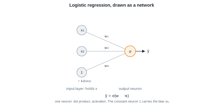 |
| + | |
| + | *Chaque arête porte un poids et le neurone applique $\sigma$ à la somme pondérée. Le neurone fixé à $1$ porte le biais : son poids est $w_0$.* |
| + | |
| + | *Remarque :* le biais reste replié dans les poids tout au long de ce module, dessiné comme un neurone constant. Le cours de [Deep Learning](/fr/Deep%20Learning) garde au contraire un vecteur de biais explicite $b^{[l]}$, et signale ce changement de convention au moment de l'introduire. |
| + | |
| + | ### 6.2.2 Insérer une couche cachée |
| + | |
| + | Rien n'oblige le neurone de sortie à lire l'entrée brute. Insérons quelques neurones entre l'entrée et la sortie, disons trois. Chacun est la même unité à produit scalaire que toujours, avec ses propres poids $w_i$ et une activation non linéaire $g$ : |
| + | |
| + | $$a_i = g(w_i^T x), \qquad i = 1, 2, 3$$ |
| - | $$\boxed{ W^{[2]}\!\left(W^{[1]} x + b^{[1]}\right) + b^{[2]} = W' x + b' }$$ |
| + | Empilons les trois vecteurs de poids $w_i^T$ comme lignes d'une matrice $W^{[1]}$, et toute la couche tient en une ligne, $a = g(W^{[1]} x)$. L'exposant entre crochets $[1]$ est nouveau, et il existe pour une raison prosaïque : le modèle a maintenant deux jeux de poids, chacun a donc besoin d'un nom. $[l]$ dit simplement à quelle couche un symbole appartient. |
| - | et la profondeur n'apporterait rien. C'est l'activation non linéaire qui rend l'empilement utile. |
| + | Le neurone de sortie n'a pas changé du tout. C'est toujours la régression logistique de la section 6.2.1, il lit simplement les trois valeurs apprises $a$, augmentées d'une constante $a_0 = 1$ (chaque couche reçoit un neurone de biais, exactement comme l'entrée), au lieu de l'entrée brute : |
| - | ## 6.2 Les couches : entrée, cachée, sortie |
| + | $$\boxed{ \hat{y} = \sigma\!\left(w^{[2]T} a\right) = \sigma\!\left(w^{[2]T}\, g(W^{[1]} x)\right) }$$ |
| - | Un neurone calcule $a = g(w^T x + b)$. Une couche empile plusieurs neurones, et un réseau empile des couches. La couche $l$ transforme les activations précédentes en nouvelles : |
| + | 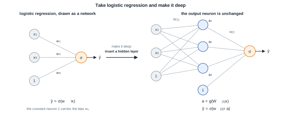 |
| - | $$\boxed{ z^{[l]} = W^{[l]} a^{[l-1]} + b^{[l]}, \quad a^{[l]} = g^{[l]}\!\left(z^{[l]}\right), \quad a^{[0]} = x, \quad \hat{y} = a^{[L]} }$$ |
| + | *Le neurone de sortie orange est identique dans les deux dessins. Rendre le modèle profond a changé ce qu'il lit : trois caractéristiques apprises $a$ au lieu du $x$ brut. Chaque couche porte son propre neurone constant $1$, dont les poids sortants sont les biais.* |
| - | La couche d'entrée contient $x$, les couches cachées apprennent des caractéristiques intermédiaires, et la couche de sortie produit la prédiction $\hat{y}$. |
| + | Deux faits sur cette insertion portent toute l'histoire. |
| + | |
| + | **L'activation cachée doit être non linéaire.** Si $g$ était l'identité, les deux couches se réduiraient à une seule application linéaire, |
| + | |
| + | $$\boxed{ W^{[2]}\!\left(W^{[1]} x\right) = W' x }$$ |
| + | |
| + | et la profondeur n'apporterait rien. C'est la non-linéarité qui rend l'empilement utile, et c'est elle qui met désormais XOR à portée. |
| + | |
| + | **La couche cachée apprend les caractéristiques.** Le neurone de sortie reste un classifieur linéaire, le travail de la couche cachée est donc de déplacer les données là où les classes deviennent linéairement séparables. Elle joue exactement le rôle des fonctions de base $\phi$ de [Régression linéaire](/fr/Machine%20Learning/04%20Linear%20regression), avec une amélioration : $\phi$ était fixée à la main avant l'entraînement, tandis que $a$ est apprise des données, de bout en bout. |
| + | |
| + | ### 6.2.3 Comment faire une prédiction ? |
| + | |
| + | Une couche cachée a fonctionné, alors répétons le geste : le vecteur $a^{[1]}$ peut alimenter une deuxième couche cachée, dont la sortie $a^{[2]}$ peut en alimenter une troisième, jusqu'à une couche de sortie qui produit $\hat{y}$. La couche $l$ possède sa matrice de poids $W^{[l]}$ (une ligne par neurone, la couche de sortie ci-dessus avait donc l'unique ligne $w^{[2]T}$) et son activation $g^{[l]}$. La largeur et la profondeur sont les boutons de capacité : plus d'unités et plus de couches donnent plus de paramètres et des frontières plus expressives, et, comme [Concepts généraux](/fr/Machine%20Learning/02%20General%20concepts) l'a prévenu, plus de place pour surapprendre. |
| 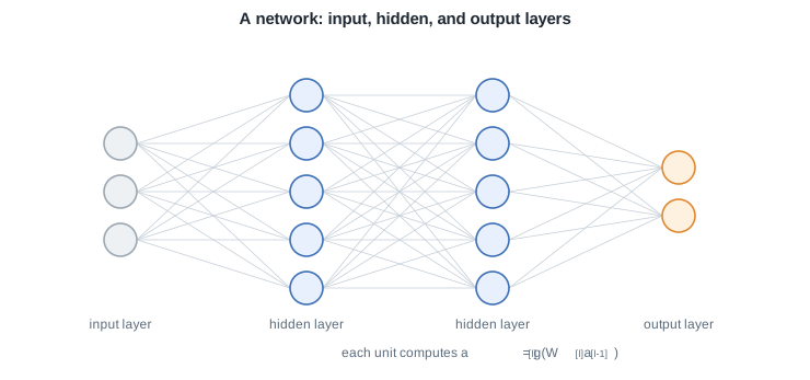 | |
| - | *Chaque arête porte un poids de $W^{[l]}$ et chaque unité ajoute un biais puis applique l'activation.* |
| + | *Chaque arête porte un poids de $W^{[l]}$. Les neurones de biais constants ne sont pas dessinés.* |
| + | |
| + | Calculer la prédiction en lisant le réseau de gauche à droite s'appelle la propagation avant, et la formule générale ne fait que redire ce que les deux dernières sections ont construit, une fois par couche : |
| + | |
| + | $$\boxed{ z^{[l]} = W^{[l]} a^{[l-1]}, \quad a^{[l]} = g^{[l]}\!\left(z^{[l]}\right), \quad a^{[0]} = x, \quad \hat{y} = a^{[L]} }$$ |
| + | |
| + | avec une convention à retenir : chaque $a^{[l]}$, comme l'entrée, se lit avec son neurone de biais $a^{[l]}_0 = 1$ ajouté en tête. Sous forme vectorisée, tout le mini-lot circule d'un coup, une opération matricielle par couche avec les exemples en colonnes, ce qui est à la fois plus clair et bien plus rapide : |
| + | |
| + | $$\boxed{ Z^{[l]} = W^{[l]} A^{[l-1]} }$$ |
| + | |
| + | La propagation avant est la première moitié de chaque pas d'entraînement. La seconde moitié, la rétropropagation, parcourt le même câblage en sens inverse (section 6.4). |
| + | |
| + | ### 6.2.4 La formule sur le graphe |
| - | *Remarque :* le biais est désormais écrit explicitement et chaque couche a sa propre matrice de poids $W^{[l]}$, contrairement à la convention antérieure qui repliait le biais dans $\theta^T x$ avec $x_0 = 1$. C'est la notation utilisée tout au long du cours de Deep Learning. |
| + | Chaque symbole de la formule de propagation avant vit quelque part sur le dessin du réseau. La figure ci-dessous les place un à un sur le plus petit réseau intéressant, deux entrées, une couche cachée de deux unités et une sortie : |
| - | ## 6.3 Couche de sortie : binaire et multiclasse |
| + | 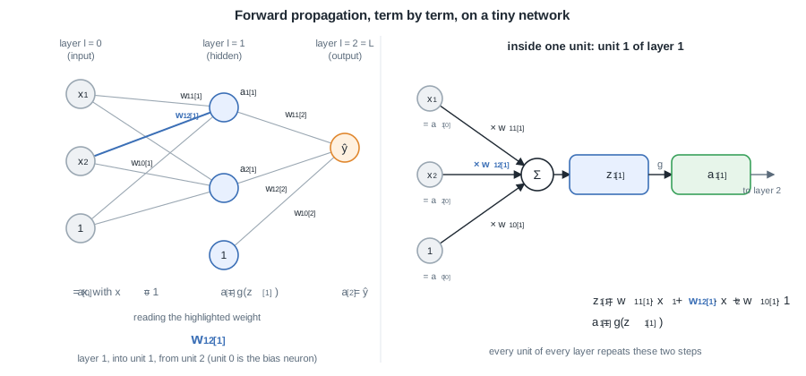 |
| - | La couche de sortie s'adapte à la tâche, en réutilisant les pertes de [Classification linéaire](/fr/Machine%20Learning/05%20Linear%20classification). Pour deux classes, une sortie sigmoïde avec l'entropie croisée binaire, et pour $k$ classes, une sortie softmax avec l'entropie croisée catégorielle : |
| + | *À gauche : l'exposant $[l]$ nomme la couche, chaque arête porte un poids $w^{[l]}_{ij}$, et les neurones fixés à $1$ portent les biais $w^{[l]}_{i0}$. À droite : à l'intérieur d'une unité, la somme pondérée donne $z^{[l]}_i$, puis l'activation $g$ la transforme en $a^{[l]}_i$.* |
| + | |
| + | | Symbole | Nom | Où il vit sur le graphe | |
| + | | --- | --- | --- | |
| + | | $l$, $L$ | indice de couche, nombre de couches | la colonne d'unités ($l = 0$ est l'entrée, ici $L = 2$) | |
| + | | $x = a^{[0]}$ | l'entrée | la colonne la plus à gauche | |
| + | | $w^{[l]}_{ij}$ | un poids | le nombre porté par une arête : vers l'unité $i$ de la couche $l$, depuis l'unité $j$ de la couche $l-1$ | |
| + | | $W^{[l]}$ | la matrice de poids de la couche $l$ | toutes les arêtes qui arrivent dans la couche $l$, une ligne par unité | |
| + | | $x_0$, $a^{[l]}_0$ | le neurone de biais | une unité fixée à $1$ dans chaque couche, dont le poids sortant $w^{[l]}_{i0}$ est le biais de l'unité $i$ | |
| + | | $z^{[l]}_i$ | la pré-activation | la somme pondérée que l'unité calcule avant d'appliquer $g$ | |
| + | | $g^{[l]}$ | la fonction d'activation | appliquée à l'intérieur de chaque unité de la couche $l$ | |
| + | | $a^{[l]}_i$ | l'activation | la valeur que l'unité envoie sur ses arêtes sortantes | |
| + | | $\hat{y} = a^{[L]}$ | la prédiction | ce qui sort de la dernière couche | |
| + | |
| + | Faisons maintenant tourner ce réseau exact avec des nombres. Prenons $x = (1, 2)$, augmenté en $(1, 1, 2)$ par le neurone de biais $x_0 = 1$, la sigmoïde du module précédent comme activation partout, avec |
| + | |
| + | $$W^{[1]} = \begin{pmatrix} 0 & 2 & -1 \\ -1 & 1 & 1 \end{pmatrix}, \qquad W^{[2]} = \begin{pmatrix} 0 & 1 & 1 \end{pmatrix}$$ |
| + | |
| + | La ligne $i$ de $W^{[1]}$ rassemble les poids des arêtes qui arrivent dans l'unité cachée $i$, biais en tête. Couche 1, unité par unité : |
| + | |
| + | $$z^{[1]}_1 = \underbrace{0}_{w^{[1]}_{10}} \cdot \underbrace{1}_{x_0} + \underbrace{2}_{w^{[1]}_{11}} \cdot \underbrace{1}_{x_1} + \underbrace{(-1)}_{w^{[1]}_{12}} \cdot \underbrace{2}_{x_2} = 0, \qquad a^{[1]}_1 = \sigma(0) = 0{,}5$$ |
| + | |
| + | $$z^{[1]}_2 = -1 \cdot 1 + 1 \cdot 1 + 1 \cdot 2 = 2, \qquad a^{[1]}_2 = \sigma(2) \approx 0{,}88$$ |
| + | |
| + | L'unité cachée 1 tombe exactement sur zéro, le point milieu de la sigmoïde, elle sort donc $0{,}5$, tandis que l'unité 2 se place haut sur la courbe. La couche de sortie répète les deux mêmes étapes, en lisant cette fois $a^{[1]} = (0{,}5,\ 0{,}88)$, augmenté en $(1,\ 0{,}5,\ 0{,}88)$ par son propre neurone de biais, au lieu de $x$ : |
| + | |
| + | $$z^{[2]} = 0 \cdot 1 + 1 \cdot 0{,}5 + 1 \cdot 0{,}88 = 1{,}38, \qquad \hat{y} = a^{[2]} = \sigma(1{,}38) \approx 0{,}80$$ |
| + | |
| + | Le réseau prédit la classe 1 avec une probabilité d'environ $0{,}80$. C'est tout ce que fait la propagation avant : multiplier par les poids des arêtes, neurone de biais compris, appliquer l'activation, à chaque unité de chaque couche. |
| + | |
| + | ## 6.3 La fonction de perte |
| + | |
| + | Le corps du réseau ignore la tâche. La tâche vit dans la dernière couche : son activation met en forme $\hat{y}$, et la perte compare $\hat{y}$ à l'étiquette, en réutilisant les pertes de [Concepts généraux](/fr/Machine%20Learning/02%20General%20concepts) et de [Classification linéaire](/fr/Machine%20Learning/05%20Linear%20classification) : |
| + | |
| + | | Tâche | Activation de sortie | Fonction de perte | |
| + | | --- | --- | --- | |
| + | | régression | identité | erreur quadratique | |
| + | | classification binaire | sigmoïde | entropie croisée binaire | |
| + | | classification multiclasse | softmax | entropie croisée catégorielle | |
| $$\boxed{ \hat{y} = \frac{1}{1 + e^{-z}} \quad\text{(binaire)} \qquad \hat{y}_c = \frac{e^{z_c}}{\sum_{j} e^{z_j}} \quad\text{(multiclasse)} }$$ | |
| - | ## 6.4 Fonctions d'activation et le problème du non-centrage en zéro |
| + | *Remarque :* ce sont exactement les têtes de neurone de [Classification linéaire](/fr/Machine%20Learning/05%20Linear%20classification). Un réseau est cette même tête posée sur des caractéristiques apprises plutôt que sur les entrées brutes. |
| + | |
| + | ## 6.4 Comment optimiser les paramètres ? |
| + | |
| + | Rien de nouveau ici non plus : entraîner un réseau suit les mêmes étapes que chaque modèle de ce cours, alors parcourons-les dans l'ordre. |
| + | |
| + | **Étape 0 : poser l'objectif.** Chercher les poids qui minimisent la perte plus un régulariseur qui les garde petits, la recette du maximum a posteriori de [Régression linéaire](/fr/Machine%20Learning/04%20Linear%20regression) : |
| + | |
| + | $$\boxed{ W^\star = \arg\min_W \; L(W) + \lambda\, R(W), \qquad R(W) = \lVert W \rVert_1 \;\text{ ou }\; \lVert W \rVert_2^2 }$$ |
| + | |
| + | **Étape 1 : choisir la perte.** C'est la section 6.3, et son tableau porte l'avertissement qui va avec : la perte et l'activation de sortie se choisissent en paire. L'entropie croisée appelle une softmax (ou une sigmoïde), l'erreur quadratique une sortie identité. |
| + | |
| + | **Étape 2 : descendre le gradient.** Mettre à jour chaque poids d'un petit pas contre son gradient, avec le taux d'apprentissage $\alpha$, exactement la descente de gradient de [Classification linéaire](/fr/Machine%20Learning/05%20Linear%20classification) : |
| + | |
| + | $$\boxed{ w^{[l]}_{ij} \leftarrow w^{[l]}_{ij} - \alpha\, \frac{\partial \left(L + \lambda R\right)}{\partial w^{[l]}_{ij}} }$$ |
| + | |
| + | **Étape 3 : obtenir le gradient par rétropropagation.** La pièce vraiment nouvelle est le calcul de ce gradient pour chaque poids d'une pile de couches. La rétropropagation y parvient avec la règle de dérivation en chaîne, en une passe avant et une passe arrière : la propagation avant met en cache chaque $z^{[l]}$ et $a^{[l]}$, puis la passe arrière propage le gradient de la perte couche par couche, de la sortie jusqu'à la première couche, en réutilisant le cache. Avec l'erreur de couche $\delta^{[l]} = \partial L / \partial z^{[l]}$, |
| + | |
| + | $$\boxed{ \delta^{[l]} = \left((W^{[l+1]})^T \delta^{[l+1]}\right) \odot g'^{[l]}\!\left(z^{[l]}\right), \qquad \frac{\partial L}{\partial W^{[l]}} = \delta^{[l]} (a^{[l-1]})^T }$$ |
| + | |
| + | Les neurones de biais s'intègrent gratuitement : constants, ils ne reçoivent aucune erreur (leur ligne de $(W^{[l+1]})^T \delta^{[l+1]}$ est simplement abandonnée), et comme $a^{[l-1]}$ contient la constante $1$, le même produit extérieur livre les gradients des biais avec le reste. |
| - | L'activation cachée est généralement la sigmoïde, la tangente hyperbolique ou l'unité de rectification linéaire : |
| + | 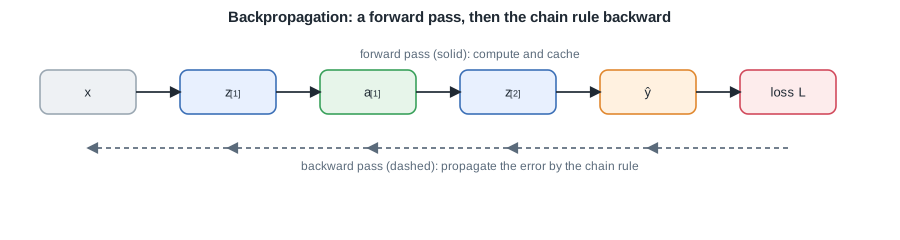 |
| + | |
| + | *La propagation avant calcule et met en cache les activations, la rétropropagation renvoie le gradient de la perte par les mêmes arêtes. La leçon [Rétropropagation](/fr/Deep%20Learning/05%20Backpropagation) du cours de Deep Learning la dérive pas à pas.* |
| + | |
| + | <details class="proof"> |
| + | <summary>Exemple complet : un pas de descente de gradient sur le petit réseau</summary> |
| + | |
| + | Reprenons le réseau de la section 6.2.4 exactement où la propagation avant l'a laissé : $\bar{x} = (1, 1, 2)$, $a^{[1]} = (0{,}5,\ 0{,}88)$, $\hat{y} = 0{,}80$, et donnons une étiquette à l'exemple : la vraie classe est $y = 0$. Prenons l'entropie croisée binaire de la section 6.3 sans régularisation ($\lambda = 0$), la perte vaut donc |
| + | |
| + | $$L = -\ln(1 - \hat{y}) = -\ln(0{,}20) \approx 1{,}61$$ |
| + | |
| + | Le réseau se trompe avec assurance, et le gradient va le lui dire. |
| + | |
| + | **En arrière à travers la couche de sortie.** Pour une sortie sigmoïde entraînée avec l'entropie croisée, l'erreur de sortie se réduit au familier $\hat{y} - y$ de [Classification linéaire](/fr/Machine%20Learning/05%20Linear%20classification) : |
| + | |
| + | $$\delta^{[2]} = \hat{y} - y = 0{,}80$$ |
| + | |
| + | Chaque poids de $W^{[2]}$ reçoit $\delta^{[2]}$ fois l'activation qu'il lit (la formule du produit extérieur, neurone de biais compris) : |
| + | |
| + | $$\frac{\partial L}{\partial W^{[2]}} = \delta^{[2]} \left(\bar{a}^{[1]}\right)^T = 0{,}80 \cdot (1,\ 0{,}5,\ 0{,}88) = (0{,}80,\ 0{,}40,\ 0{,}70)$$ |
| + | |
| + | **En arrière à travers la couche cachée.** Chaque unité cachée prend sa part de l'erreur à travers son poids sortant, fois sa propre pente $\sigma'(z) = \sigma(z)(1 - \sigma(z))$ : |
| + | |
| + | $$\delta^{[1]}_1 = w^{[2]}_{11}\, \delta^{[2]}\, \sigma'(0) = 1 \cdot 0{,}80 \cdot 0{,}25 = 0{,}20, \qquad \delta^{[1]}_2 = 1 \cdot 0{,}80 \cdot 0{,}10 = 0{,}08$$ |
| + | |
| + | (le neurone de biais constant ne prend aucune erreur, et notez la petite pente $0{,}10$ de l'unité 2 : la section 6.5 y reviendra). Puis le même produit extérieur contre $\bar{x} = (1, 1, 2)$ : |
| + | |
| + | $$\frac{\partial L}{\partial W^{[1]}} = \delta^{[1]}\, \bar{x}^T = \begin{pmatrix} 0{,}20 & 0{,}20 & 0{,}40 \\ 0{,}08 & 0{,}08 & 0{,}16 \end{pmatrix}$$ |
| + | |
| + | **La mise à jour.** L'étape 2 avec un $\alpha = 1$ volontairement grand, pour rendre le mouvement visible : |
| + | |
| + | $$W^{[2]} \leftarrow (0,\ 1,\ 1) - (0{,}80,\ 0{,}40,\ 0{,}70) = (-0{,}80,\ 0{,}60,\ 0{,}30)$$ |
| + | |
| + | $$W^{[1]} \leftarrow \begin{pmatrix} 0 & 2 & -1 \\ -1 & 1 & 1 \end{pmatrix} - \begin{pmatrix} 0{,}20 & 0{,}20 & 0{,}40 \\ 0{,}08 & 0{,}08 & 0{,}16 \end{pmatrix} = \begin{pmatrix} -0{,}20 & 1{,}80 & -1{,}40 \\ -1{,}08 & 0{,}92 & 0{,}84 \end{pmatrix}$$ |
| + | |
| + | **Est-ce que ça a aidé ?** Relançons la propagation avant avec les nouveaux poids : $z^{[1]} = (-1{,}20,\ 1{,}52)$, $a^{[1]} = (0{,}23,\ 0{,}82)$, $z^{[2]} = -0{,}42$, et |
| + | |
| + | $$\hat{y} = \sigma(-0{,}42) \approx 0{,}40, \qquad L = -\ln(1 - 0{,}40) \approx 0{,}51$$ |
| + | |
| + | Un seul pas, et la prédiction de la classe 1 est passée de $0{,}80$ à $0{,}40$, la perte de $1{,}61$ à $0{,}51$. L'entraînement, c'est cette boucle, répétée sur les mini-lots jusqu'à ce que la perte se stabilise. |
| + | |
| + | </details> |
| + | |
| + | ## 6.5 La disparition du gradient |
| + | |
| + | La formule de rétropropagation cache un piège. À chaque couche traversée, l'erreur $\delta^{[l]}$ est multipliée par la pente locale $g'(z^{[l]})$, si bien que le gradient qui atteint la couche 1 contient un tel facteur par couche. Avec des activations sigmoïdes, ces facteurs sont petits par construction : |
| + | |
| + | $$\boxed{ \sigma'(z) = \sigma(z)\left(1 - \sigma(z)\right) \le \tfrac{1}{4} }$$ |
| + | |
| + | Le résultat est la disparition du gradient : les couches proches de la sortie apprennent, celles proches de l'entrée ne reçoivent presque rien et bougent à peine. Les réseaux sigmoïdes profonds stagnent, et le remède n'est pas un meilleur optimiseur, c'est une meilleure activation (section 6.6). |
| + | |
| + | <details class="proof"> |
| + | <summary>Preuve : le gradient rétrécit géométriquement avec la profondeur</summary> |
| + | |
| + | **Étape 1 : la pente de la sigmoïde ne dépasse jamais $1/4$.** Dérivons $\sigma(z) = (1 + e^{-z})^{-1}$ avec la règle de dérivation en chaîne : |
| + | |
| + | $$\sigma'(z) = \frac{e^{-z}}{\left(1 + e^{-z}\right)^2} = \frac{1}{1 + e^{-z}} \cdot \frac{e^{-z}}{1 + e^{-z}} = \sigma(z)\left(1 - \sigma(z)\right)$$ |
| + | |
| + | Posons $s = \sigma(z) \in (0, 1)$. Le produit $s(1 - s)$ est une parabole tournée vers le bas, maximale en $s = \tfrac{1}{2}$ où elle vaut $\tfrac{1}{4}$. La borne tient donc, avec égalité seulement en $z = 0$, et la saturation aggrave tout : dans l'exemple détaillé de la section 6.2.4, l'unité cachée 2 se trouve à $\sigma(2) \approx 0{,}88$, où la pente est déjà tombée à $0{,}88 \cdot 0{,}12 \approx 0{,}10$. |
| + | |
| + | **Étape 2 : la rétropropagation multiplie ces pentes.** Prenons le réseau profond le plus simple, une chaîne de $L$ couches à une unité chacune, où chaque quantité est un scalaire. En appliquant la règle de dérivation en chaîne de la sortie vers la couche 1, chaque couche traversée apporte le facteur $\partial z^{[l]} / \partial z^{[l-1]} = w^{[l]}\, \sigma'(z^{[l-1]})$ : |
| + | |
| + | $$\frac{\partial L}{\partial z^{[1]}} = \frac{\partial L}{\partial z^{[L]}} \prod_{l=2}^{L} w^{[l]}\, \sigma'(z^{[l-1]})$$ |
| + | |
| + | Avec des poids de taille typique $|w^{[l]}| \le 1$, chaque facteur vaut au plus $\tfrac{1}{4}$ en valeur absolue, donc |
| + | |
| + | $$\boxed{ \left|\frac{\partial L}{\partial z^{[1]}}\right| \le \left(\tfrac{1}{4}\right)^{L-1} \left|\frac{\partial L}{\partial z^{[L]}}\right| }$$ |
| + | |
| + | Dix couches rétrécissent déjà le gradient d'environ $10^{-6}$. Le cas matriciel complet est la récursion de la section 6.4, avec la même conclusion. $\blacksquare$ |
| + | |
| + | </details> |
| + | |
| + | Des poids bien plus grands que $1$ ne font qu'échanger le problème contre son image miroir, l'explosion du gradient. La leçon [Initialisation et disparition du gradient](/fr/Deep%20Learning/07%20Initialization%20and%20vanishing%20gradients) du cours de Deep Learning en donne le traitement complet. |
| + | |
| + | ## 6.6 Les fonctions d'activation |
| + | |
| + | Alors, quelle activation choisir pour $g$ ? Les candidates, dans l'ordre où l'histoire les a essayées : |
| $$\boxed{ \sigma(z) = \frac{1}{1 + e^{-z}}, \qquad \tanh(z), \qquad \mathrm{ReLU}(z) = \max(0, z) }$$ | |
| - | La sigmoïde sature dans ses queues, et ses sorties ne sont jamais négatives, donc les poids entrants d'une unité reçoivent des gradients de même signe et les mises à jour zigzaguent. La $\tanh$, centrée en zéro, supprime ce biais, et ReLU évite complètement la saturation du côté positif, ce qui en fait le choix par défaut courant. |
| + | La sigmoïde sature dans ses deux queues, exactement ce que la section 6.5 vient de punir, et ses sorties ne sont jamais négatives, donc les poids entrants d'une unité reçoivent des gradients de même signe et les mises à jour zigzaguent. La $\tanh$, centrée en zéro, supprime ce biais mais sature encore. ReLU garde une pente d'exactement $1$ sur tout son côté positif, les facteurs rétrécissants de la section 6.5 disparaissent donc, et elle ne coûte presque rien à calculer. C'est pourquoi elle est aujourd'hui l'activation cachée par défaut. |
|  | |
| *La tanh est centrée en zéro alors que la sigmoïde ne l'est pas, et ReLU reste linéaire pour les entrées positives.* | |
| - | ## 6.5 Règle de dérivation en chaîne et rétropropagation |
| + | ReLU a un angle mort : une unité dont l'entrée reste négative sort $0$, a une pente de $0$ et cesse d'apprendre, une unité morte. Des variantes comme Leaky ReLU, $\max(0{,}01\, z, z)$, et ELU gardent une petite pente du côté négatif pour l'éviter. En pratique : commencer avec ReLU, essayer ses variantes si des unités meurent, et réserver la sigmoïde là où la section 6.3 en a besoin, à la sortie d'un classifieur binaire. La leçon [Fonctions d'activation](/fr/Deep%20Learning/03%20Activation%20functions) du cours de Deep Learning les compare toutes. |
| - | L'entraînement minimise la perte par descente de gradient, qui a besoin de son gradient par rapport à chaque poids. La rétropropagation les calcule tous en une passe avant et une passe arrière : la passe avant met en cache chaque $z^{[l]}$ et $a^{[l]}$, puis la passe arrière applique la règle de dérivation en chaîne de la perte jusqu'à la première couche, en réutilisant le cache. Avec l'erreur de couche $\delta^{[l]} = \partial L / \partial z^{[l]}$, |
| + | ## 6.7 Les bonnes pratiques |
| - | $$\boxed{ \delta^{[l]} = \left((W^{[l+1]})^T \delta^{[l+1]}\right) \odot g'^{[l]}\!\left(z^{[l]}\right), \qquad \frac{\partial L}{\partial W^{[l]}} = \delta^{[l]} (a^{[l-1]})^T }$$ |
| + | Cinq habitudes font la différence entre un réseau qui s'entraîne et un réseau qui stagne. |
| - |  |
| + | **Entraîner par mini-lots.** [Classification linéaire](/fr/Machine%20Learning/05%20Linear%20classification) offrait deux extrêmes, le lot complet ou un seul exemple par pas. Les réseaux s'entraînent par mini-lots, un petit lot par pas : un gradient assez précis pour progresser, un pas assez bon marché pour en faire des milliers, et la propagation avant vectorisée de la section 6.2.3 traite tout le mini-lot en un produit matriciel par couche. |
| + | |
| + | **Initialiser avec soin.** Des poids tous égaux feraient calculer la même chose à chaque unité d'une couche pour toujours, on démarre donc petit et aléatoire pour briser la symétrie. L'échelle compte aussi : trop petit et les activations rétrécissent vers zéro couche après couche, trop grand et elles saturent. Mettre la variance à l'échelle du nombre d'entrées de l'unité, Xavier pour tanh, He pour ReLU. |
| + | |
| + | **Centrer et normaliser les entrées.** Standardiser chaque caractéristique (soustraire sa moyenne, diviser par son écart-type), pour qu'aucune ne domine les premiers produits scalaires et que le zigzag des entrées toutes positives de la section 6.6 disparaisse dès la première couche. |
| + | |
| + | **Dropout.** Mettre à zéro au hasard une fraction des unités pendant l'entraînement pour qu'aucune ne puisse s'appuyer sur ses voisines, un régulariseur dans l'esprit de [Concepts généraux](/fr/Machine%20Learning/02%20General%20concepts). En prédiction, toutes les unités restent actives et les sorties sont mises à l'échelle par la probabilité de conservation, ce qui approche la moyenne des nombreux réseaux amincis ([Régularisation et dropout](/fr/Deep%20Learning/09%20Regularization%20and%20dropout)). |
| + | |
| + | **Vérifier avant d'entraîner longtemps.** Un classifieur à $K$ classes fraîchement initialisé doit démarrer près de la perte $\ln K$ (environ $2{,}3$ pour $K = 10$). Un minuscule jeu d'entraînement doit être facile à surapprendre : si le réseau n'y arrive pas, le code est cassé. Surveiller les courbes d'entraînement et de validation. Et comme la rétropropagation est source d'erreurs, comparer son gradient analytique à une estimation numérique par différences finies : |
| + | |
| + | $$\boxed{ \frac{\partial L}{\partial w} \approx \frac{L(w + \varepsilon) - L(w - \varepsilon)}{2\varepsilon} }$$ |
| + | |
| + | ## 6.8 La descente de gradient améliorée |
| + | |
| + | La descente de gradient brute prend le pas le plus pentu et rien de plus, et trois paysages la mettent en échec : les plateaux, où la pente est presque nulle et le progrès s'arrête, les points de selle (fréquents en haute dimension), où le gradient est exactement nul sans être un minimum, et les ravins, pentus dans une direction et doux dans l'autre, où le pas oscille entre les parois en rampant le long du fond. |
| - | *La leçon [Rétropropagation](/fr/Deep%20Learning/05%20Backpropagation) du cours de Deep Learning la dérive pas à pas.* |
| + | **Le momentum** traite la mise à jour comme une vitesse avec frottement : les gradients s'accumulent, les directions persistantes prennent de la vitesse, les directions oscillantes s'annulent : |
| - | ## 6.6 L'entraînement en pratique |
| + | $$\boxed{ v \leftarrow \rho\, v + \nabla_W L, \qquad W \leftarrow W - \alpha\, v }$$ |
| - | - **Mini-lots.** Estimer le gradient sur un petit lot d'exemples à la fois, un compromis entre le lot complet (précis mais lent) et un seul exemple (bruité mais peu coûteux). |
| - | - **Disparition du gradient.** À travers de nombreuses couches qui saturent, le gradient rétropropagé est un produit de petits facteurs et tend vers zéro, si bien que les premières couches n'apprennent presque pas. Les activations ReLU et une initialisation soignée le maintiennent vivant. |
| - | - **Initialisation.** Démarrer les poids petits et aléatoires pour briser la symétrie, en mettant la variance à l'échelle du nombre d'entrées (Xavier ou He), pour que les signaux ne s'évanouissent ni n'explosent avec la profondeur. |
| - | - **Dropout.** Mettre à zéro au hasard une fraction des unités pendant l'entraînement. Cela empêche les unités de se co-adapter et agit comme un régulariseur, dans l'esprit de la régularisation de [Concepts généraux](/fr/Machine%20Learning/02%20General%20concepts). |
| + | avec un frottement $\rho$ typiquement autour de $0{,}9$. |
| - | ## 6.7 Tests de validité et vectorisation |
| + | **RMSProp** donne à chaque paramètre son propre pas, en divisant par une moyenne glissante de l'amplitude du gradient, ce qui tempère les directions pentues et accélère les plates : |
| - | La rétropropagation est source d'erreurs, alors on compare le gradient analytique à une estimation numérique par différences finies : |
| + | $$\boxed{ m \leftarrow \beta\, m + (1 - \beta) \left(\nabla_W L\right)^2, \qquad W \leftarrow W - \frac{\alpha}{\sqrt{m} + \varepsilon}\, \nabla_W L }$$ |
| - | $$\boxed{ \frac{\partial L}{\partial \theta} \approx \frac{L(\theta + \varepsilon) - L(\theta - \varepsilon)}{2\varepsilon} }$$ |
| + | **Adam** combine les deux idées, une vitesse pour la direction et une échelle par paramètre pour le pas (la version complète corrige aussi un biais de démarrage dans $v$ et $m$), et c'est l'optimiseur par défaut en pratique : |
| - | et on implémente les passes sous forme vectorisée, une opération matricielle par couche sur tout le mini-lot (les colonnes sont les exemples), ce qui est à la fois plus clair et bien plus rapide : |
| + | $$\boxed{ v \leftarrow \beta_1 v + (1 - \beta_1)\, \nabla_W L, \qquad m \leftarrow \beta_2 m + (1 - \beta_2) \left(\nabla_W L\right)^2, \qquad W \leftarrow W - \alpha\, \frac{v}{\sqrt{m} + \varepsilon} }$$ |
| - | $$\boxed{ Z^{[l]} = W^{[l]} A^{[l-1]} + b^{[l]} }$$ |
| + | Deux habitudes complètent le tableau : faire décroître le taux d'apprentissage au fil de l'entraînement, et se rappeler que ces trois méthodes consomment toujours les gradients par mini-lots de la section 6.7, elles ne font que mieux les dépenser. La leçon [Optimisation](/fr/Deep%20Learning/06%20Optimization) du cours de Deep Learning les dérive une à une et ajoute les calendriers de taux d'apprentissage. |
| *Ce module est la porte d'entrée du cours de [Deep Learning](/fr/Deep%20Learning), qui développe pleinement les architectures, les optimiseurs, l'initialisation, la normalisation et la régularisation. Le module suivant revient aux modèles linéaires sous un nouvel angle, le classifieur à marge maximale.* | |
| /dev/null .. fr/Machine Learning/06 Multilayer neural networks/forward-notation.svg | |
| @@ 0,0 1,96 @@ | |
| + | <svg xmlns="http://www.w3.org/2000/svg" viewBox="0 0 900 420" width="900" height="420" font-family="Helvetica, Arial, sans-serif"> |
| + | <defs> |
| + | <marker id="arrow" viewBox="0 0 10 10" refX="8.5" refY="5" markerWidth="7" markerHeight="7" orient="auto-start-reverse"><path d="M0 0L10 5L0 10z" fill="#1f2933"/></marker> |
| + | <marker id="arrowmuted" viewBox="0 0 10 10" refX="8.5" refY="5" markerWidth="7" markerHeight="7" orient="auto-start-reverse"><path d="M0 0L10 5L0 10z" fill="#5b6b7b"/></marker> |
| + | </defs> |
| + | <rect width="900" height="420" fill="#ffffff"/> |
| + | <text x="450" y="22" font-size="15" font-weight="600" fill="#1f2933" text-anchor="middle">Forward propagation, term by term, on a tiny network</text> |
| + | |
| + | <!-- Panel A: annotated network --> |
| + | <text x="90" y="52" font-size="11" fill="#5b6b7b" text-anchor="middle">layer l = 0</text> |
| + | <text x="90" y="66" font-size="11" fill="#5b6b7b" text-anchor="middle">(input)</text> |
| + | <text x="250" y="52" font-size="11" fill="#5b6b7b" text-anchor="middle">layer l = 1</text> |
| + | <text x="250" y="66" font-size="11" fill="#5b6b7b" text-anchor="middle">(hidden)</text> |
| + | <text x="385" y="52" font-size="11" fill="#5b6b7b" text-anchor="middle">layer l = 2 = L</text> |
| + | <text x="385" y="66" font-size="11" fill="#5b6b7b" text-anchor="middle">(output)</text> |
| + | |
| + | <line x1="105.9" y1="106.5" x2="234.1" y2="118.5" stroke="#9aa7b2" stroke-width="1.1"/> |
| + | <line x1="103.4" y1="113.8" x2="236.6" y2="201.2" stroke="#9aa7b2" stroke-width="1.1"/> |
| + | <line x1="105.7" y1="182.9" x2="234.3" y2="207.1" stroke="#9aa7b2" stroke-width="1.1"/> |
| + | <line x1="105" y1="174.4" x2="235" y2="125.6" stroke="#3b6fb6" stroke-width="2"/> |
| + | <line x1="102.2" y1="244.7" x2="237.8" y2="130.3" stroke="#9aa7b2" stroke-width="1.1"/> |
| + | <line x1="105.4" y1="250.7" x2="234.6" y2="214.3" stroke="#9aa7b2" stroke-width="1.1"/> |
| + | <line x1="265.2" y1="125.1" x2="369.8" y2="159.9" stroke="#9aa7b2" stroke-width="1.1"/> |
| + | <line x1="265.2" y1="204.9" x2="369.8" y2="170.1" stroke="#9aa7b2" stroke-width="1.1"/> |
| + | <line x1="262" y1="274.4" x2="373" y2="175.6" stroke="#9aa7b2" stroke-width="1.1"/> |
| + | |
| + | <text x="205" y="110" font-size="11" fill="#1f2933" text-anchor="middle">w<tspan baseline-shift="sub" font-size="8px">11</tspan><tspan baseline-shift="super" font-size="8px">[1]</tspan></text> |
| + | <text x="200" y="132" font-size="11" font-weight="600" fill="#3b6fb6" text-anchor="middle">w<tspan baseline-shift="sub" font-size="8px">12</tspan><tspan baseline-shift="super" font-size="8px">[1]</tspan></text> |
| + | <text x="150" y="185" font-size="11" fill="#1f2933" text-anchor="middle">w<tspan baseline-shift="sub" font-size="8px">10</tspan><tspan baseline-shift="super" font-size="8px">[1]</tspan></text> |
| + | <text x="322" y="131" font-size="11" fill="#1f2933" text-anchor="middle">w<tspan baseline-shift="sub" font-size="8px">11</tspan><tspan baseline-shift="super" font-size="8px">[2]</tspan></text> |
| + | <text x="300" y="214" font-size="11" fill="#1f2933" text-anchor="middle">w<tspan baseline-shift="sub" font-size="8px">12</tspan><tspan baseline-shift="super" font-size="8px">[2]</tspan></text> |
| + | <text x="332" y="241" font-size="11" fill="#1f2933" text-anchor="middle">w<tspan baseline-shift="sub" font-size="8px">10</tspan><tspan baseline-shift="super" font-size="8px">[2]</tspan></text> |
| + | |
| + | <circle cx="90" cy="105" r="16" fill="#eef1f4" stroke="#9aa7b2" stroke-width="1.6"/> |
| + | <text x="90" y="109" font-size="12" fill="#1f2933" text-anchor="middle">x<tspan baseline-shift="sub" font-size="9px">1</tspan></text> |
| + | <circle cx="90" cy="180" r="16" fill="#eef1f4" stroke="#9aa7b2" stroke-width="1.6"/> |
| + | <text x="90" y="184" font-size="12" fill="#1f2933" text-anchor="middle">x<tspan baseline-shift="sub" font-size="9px">2</tspan></text> |
| + | <circle cx="90" cy="255" r="16" fill="#eef1f4" stroke="#9aa7b2" stroke-width="1.6"/> |
| + | <text x="90" y="259" font-size="12" fill="#1f2933" text-anchor="middle">1</text> |
| + | <circle cx="250" cy="120" r="16" fill="#e8f0fe" stroke="#3b6fb6" stroke-width="1.6"/> |
| + | <circle cx="250" cy="210" r="16" fill="#e8f0fe" stroke="#3b6fb6" stroke-width="1.6"/> |
| + | <circle cx="250" cy="285" r="16" fill="#e8f0fe" stroke="#3b6fb6" stroke-width="1.6"/> |
| + | <text x="250" y="289" font-size="12" fill="#1f2933" text-anchor="middle">1</text> |
| + | <circle cx="385" cy="165" r="16" fill="#fff1e0" stroke="#e0872e" stroke-width="1.6"/> |
| + | <text x="385" y="170" font-size="13" fill="#1f2933" text-anchor="middle">ŷ</text> |
| + | |
| + | <text x="268" y="106" font-size="11" fill="#1f2933">a<tspan baseline-shift="sub" font-size="8px">1</tspan><tspan baseline-shift="super" font-size="8px">[1]</tspan></text> |
| + | <text x="268" y="192" font-size="11" fill="#1f2933">a<tspan baseline-shift="sub" font-size="8px">2</tspan><tspan baseline-shift="super" font-size="8px">[1]</tspan></text> |
| + | |
| + | <text x="90" y="330" font-size="12" fill="#5b6b7b" text-anchor="middle">a<tspan baseline-shift="super" font-size="9px">[0]</tspan> = x, with x<tspan baseline-shift="sub" font-size="9px">0</tspan> = 1</text> |
| + | <text x="250" y="330" font-size="12" fill="#5b6b7b" text-anchor="middle">a<tspan baseline-shift="super" font-size="9px">[1]</tspan> = g(z<tspan baseline-shift="super" font-size="9px">[1]</tspan>)</text> |
| + | <text x="385" y="330" font-size="12" fill="#5b6b7b" text-anchor="middle">a<tspan baseline-shift="super" font-size="9px">[2]</tspan> = ŷ</text> |
| + | |
| + | <text x="220" y="358" font-size="11" fill="#5b6b7b" text-anchor="middle">reading the highlighted weight</text> |
| + | <text x="220" y="384" font-size="17" font-weight="600" fill="#3b6fb6" text-anchor="middle">w<tspan baseline-shift="sub" font-size="11px">12</tspan><tspan baseline-shift="super" font-size="11px">[1]</tspan></text> |
| + | <text x="220" y="404" font-size="11" fill="#5b6b7b" text-anchor="middle">layer 1, into unit 1, from unit 2 (unit 0 is the bias neuron)</text> |
| + | |
| + | <line x1="425" y1="40" x2="425" y2="405" stroke="#e3e8ee" stroke-width="1"/> |
| + | |
| + | <!-- Panel B: inside one unit --> |
| + | <text x="665" y="56" font-size="13" font-weight="600" fill="#1f2933" text-anchor="middle">inside one unit: unit 1 of layer 1</text> |
| + | |
| + | <line x1="491.4" y1="118.1" x2="585.3" y2="184.6" stroke="#1f2933" stroke-width="1.4" marker-end="url(#arrow)"/> |
| + | <line x1="494" y1="195" x2="582" y2="195" stroke="#1f2933" stroke-width="1.4" marker-end="url(#arrow)"/> |
| + | <line x1="491.4" y1="271.9" x2="585.3" y2="205.4" stroke="#1f2933" stroke-width="1.4" marker-end="url(#arrow)"/> |
| + | <text x="556" y="146" font-size="11" fill="#1f2933" text-anchor="middle">× w<tspan baseline-shift="sub" font-size="8px">11</tspan><tspan baseline-shift="super" font-size="8px">[1]</tspan></text> |
| + | <text x="538" y="187" font-size="11" font-weight="600" fill="#3b6fb6" text-anchor="middle">× w<tspan baseline-shift="sub" font-size="8px">12</tspan><tspan baseline-shift="super" font-size="8px">[1]</tspan></text> |
| + | <text x="556" y="254" font-size="11" fill="#1f2933" text-anchor="middle">× w<tspan baseline-shift="sub" font-size="8px">10</tspan><tspan baseline-shift="super" font-size="8px">[1]</tspan></text> |
| + | |
| + | <circle cx="480" cy="110" r="14" fill="#eef1f4" stroke="#9aa7b2" stroke-width="1.6"/> |
| + | <text x="480" y="114" font-size="11" fill="#1f2933" text-anchor="middle">x<tspan baseline-shift="sub" font-size="8px">1</tspan></text> |
| + | <text x="480" y="142" font-size="10" fill="#5b6b7b" text-anchor="middle">= a<tspan baseline-shift="sub" font-size="7px">1</tspan><tspan baseline-shift="super" font-size="7px">[0]</tspan></text> |
| + | <circle cx="480" cy="195" r="14" fill="#eef1f4" stroke="#9aa7b2" stroke-width="1.6"/> |
| + | <text x="480" y="199" font-size="11" fill="#1f2933" text-anchor="middle">x<tspan baseline-shift="sub" font-size="8px">2</tspan></text> |
| + | <text x="480" y="227" font-size="10" fill="#5b6b7b" text-anchor="middle">= a<tspan baseline-shift="sub" font-size="7px">2</tspan><tspan baseline-shift="super" font-size="7px">[0]</tspan></text> |
| + | <circle cx="480" cy="280" r="14" fill="#eef1f4" stroke="#9aa7b2" stroke-width="1.6"/> |
| + | <text x="480" y="284" font-size="11" fill="#1f2933" text-anchor="middle">1</text> |
| + | <text x="480" y="312" font-size="10" fill="#5b6b7b" text-anchor="middle">= a<tspan baseline-shift="sub" font-size="7px">0</tspan><tspan baseline-shift="super" font-size="7px">[0]</tspan></text> |
| + | |
| + | <circle cx="600" cy="195" r="18" fill="#ffffff" stroke="#1f2933" stroke-width="1.6"/> |
| + | <text x="600" y="200" font-size="14" fill="#1f2933" text-anchor="middle">Σ</text> |
| + | |
| + | <line x1="618" y1="195" x2="636" y2="195" stroke="#1f2933" stroke-width="1.4" marker-end="url(#arrow)"/> |
| + | <rect x="636" y="173" width="88" height="44" rx="8" fill="#e8f0fe" stroke="#3b6fb6" stroke-width="1.6"/> |
| + | <text x="680" y="199" font-size="13" fill="#1f2933" text-anchor="middle">z<tspan baseline-shift="sub" font-size="9px">1</tspan><tspan baseline-shift="super" font-size="9px">[1]</tspan></text> |
| + | <line x1="724" y1="195" x2="750" y2="195" stroke="#1f2933" stroke-width="1.4" marker-end="url(#arrow)"/> |
| + | <text x="737" y="187" font-size="11" fill="#5b6b7b" text-anchor="middle">g</text> |
| + | <rect x="750" y="173" width="88" height="44" rx="8" fill="#e7f5ea" stroke="#38a05a" stroke-width="1.6"/> |
| + | <text x="794" y="199" font-size="13" fill="#1f2933" text-anchor="middle">a<tspan baseline-shift="sub" font-size="9px">1</tspan><tspan baseline-shift="super" font-size="9px">[1]</tspan></text> |
| + | <line x1="838" y1="195" x2="864" y2="195" stroke="#5b6b7b" stroke-width="1.3" marker-end="url(#arrowmuted)"/> |
| + | <text x="851" y="216" font-size="10" fill="#5b6b7b" text-anchor="middle">to layer 2</text> |
| + | |
| + | <text x="665" y="340" font-size="13" fill="#1f2933" text-anchor="middle">z<tspan baseline-shift="sub" font-size="9px">1</tspan><tspan baseline-shift="super" font-size="9px">[1]</tspan> = w<tspan baseline-shift="sub" font-size="9px">11</tspan><tspan baseline-shift="super" font-size="9px">[1]</tspan> · x<tspan baseline-shift="sub" font-size="9px">1</tspan> + <tspan font-weight="600" fill="#3b6fb6">w<tspan baseline-shift="sub" font-size="9px">12</tspan><tspan baseline-shift="super" font-size="9px">[1]</tspan></tspan> · x<tspan baseline-shift="sub" font-size="9px">2</tspan> + w<tspan baseline-shift="sub" font-size="9px">10</tspan><tspan baseline-shift="super" font-size="9px">[1]</tspan> · 1</text> |
| + | <text x="665" y="364" font-size="13" fill="#1f2933" text-anchor="middle">a<tspan baseline-shift="sub" font-size="9px">1</tspan><tspan baseline-shift="super" font-size="9px">[1]</tspan> = g(z<tspan baseline-shift="sub" font-size="9px">1</tspan><tspan baseline-shift="super" font-size="9px">[1]</tspan>)</text> |
| + | <text x="665" y="396" font-size="11" fill="#5b6b7b" text-anchor="middle">every unit of every layer repeats these two steps</text> |
| + | </svg> |
| /dev/null .. fr/Machine Learning/06 Multilayer neural networks/logreg-network.svg | |
| @@ 0,0 1,32 @@ | |
| + | <svg xmlns="http://www.w3.org/2000/svg" viewBox="0 0 740 345" width="740" height="345" font-family="Helvetica, Arial, sans-serif"> |
| + | <defs> |
| + | <marker id="arrow" viewBox="0 0 10 10" refX="8.5" refY="5" markerWidth="7" markerHeight="7" orient="auto-start-reverse"><path d="M0 0L10 5L0 10z" fill="#1f2933"/></marker> |
| + | </defs> |
| + | <rect width="740" height="345" fill="#ffffff"/> |
| + | <text x="370" y="22" font-size="15" font-weight="600" fill="#1f2933" text-anchor="middle">Logistic regression, drawn as a network</text> |
| + | |
| + | <line x1="284.7" y1="106.4" x2="413.5" y2="162.8" stroke="#9aa7b2" stroke-width="1.1"/> |
| + | <line x1="286" y1="170" x2="412" y2="170" stroke="#9aa7b2" stroke-width="1.1"/> |
| + | <line x1="284.7" y1="233.6" x2="413.5" y2="177.2" stroke="#9aa7b2" stroke-width="1.1"/> |
| + | <text x="349" y="124" font-size="11" fill="#1f2933" text-anchor="middle">w<tspan baseline-shift="sub" font-size="8px">1</tspan></text> |
| + | <text x="349" y="162" font-size="11" fill="#1f2933" text-anchor="middle">w<tspan baseline-shift="sub" font-size="8px">2</tspan></text> |
| + | <text x="349" y="222" font-size="11" fill="#1f2933" text-anchor="middle">w<tspan baseline-shift="sub" font-size="8px">0</tspan></text> |
| + | |
| + | <circle cx="270" cy="100" r="16" fill="#eef1f4" stroke="#9aa7b2" stroke-width="1.6"/> |
| + | <text x="270" y="104" font-size="12" fill="#1f2933" text-anchor="middle">x<tspan baseline-shift="sub" font-size="9px">1</tspan></text> |
| + | <circle cx="270" cy="170" r="16" fill="#eef1f4" stroke="#9aa7b2" stroke-width="1.6"/> |
| + | <text x="270" y="174" font-size="12" fill="#1f2933" text-anchor="middle">x<tspan baseline-shift="sub" font-size="9px">2</tspan></text> |
| + | <circle cx="270" cy="240" r="16" fill="#eef1f4" stroke="#9aa7b2" stroke-width="1.6"/> |
| + | <text x="270" y="244" font-size="12" fill="#1f2933" text-anchor="middle">1</text> |
| + | <text x="270" y="272" font-size="10" fill="#5b6b7b" text-anchor="middle">x<tspan baseline-shift="sub" font-size="7px">0</tspan> = 1 (bias)</text> |
| + | <circle cx="430" cy="170" r="18" fill="#fff1e0" stroke="#e0872e" stroke-width="1.6"/> |
| + | <text x="430" y="175" font-size="13" fill="#1f2933" text-anchor="middle">σ</text> |
| + | <line x1="448" y1="170" x2="478" y2="170" stroke="#1f2933" stroke-width="1.4" marker-end="url(#arrow)"/> |
| + | <text x="490" y="174" font-size="13" fill="#1f2933" text-anchor="middle">ŷ</text> |
| + | |
| + | <text x="270" y="298" font-size="12" fill="#5b6b7b" text-anchor="middle">input layer: holds x</text> |
| + | <text x="430" y="298" font-size="12" fill="#5b6b7b" text-anchor="middle">output neuron</text> |
| + | |
| + | <text x="370" y="322" font-size="13" fill="#1f2933" text-anchor="middle">ŷ = σ(w<tspan baseline-shift="super" font-size="9px">T</tspan>x)</text> |
| + | <text x="370" y="340" font-size="11" fill="#5b6b7b" text-anchor="middle">one neuron: dot product, activation. The constant neuron 1 carries the bias w₀</text> |
| + | </svg> |
| /dev/null .. fr/Machine Learning/06 Multilayer neural networks/make-it-deep.svg | |
| @@ 0,0 1,80 @@ | |
| + | <svg xmlns="http://www.w3.org/2000/svg" viewBox="0 0 900 380" width="900" height="380" font-family="Helvetica, Arial, sans-serif"> |
| + | <defs> |
| + | <marker id="arrow" viewBox="0 0 10 10" refX="8.5" refY="5" markerWidth="7" markerHeight="7" orient="auto-start-reverse"><path d="M0 0L10 5L0 10z" fill="#1f2933"/></marker> |
| + | </defs> |
| + | <rect width="900" height="380" fill="#ffffff"/> |
| + | <text x="450" y="22" font-size="15" font-weight="600" fill="#1f2933" text-anchor="middle">Take logistic regression and make it deep</text> |
| + | |
| + | <!-- Panel 1: logistic regression as a network --> |
| + | <text x="185" y="48" font-size="13" font-weight="600" fill="#1f2933" text-anchor="middle">logistic regression, drawn as a network</text> |
| + | |
| + | <line x1="124.3" y1="117.2" x2="243.9" y2="177" stroke="#9aa7b2" stroke-width="1.1"/> |
| + | <line x1="126" y1="185" x2="242" y2="185" stroke="#9aa7b2" stroke-width="1.1"/> |
| + | <line x1="124.3" y1="252.8" x2="243.9" y2="193" stroke="#9aa7b2" stroke-width="1.1"/> |
| + | <text x="184" y="136" font-size="11" fill="#1f2933" text-anchor="middle">w<tspan baseline-shift="sub" font-size="8px">1</tspan></text> |
| + | <text x="184" y="177" font-size="11" fill="#1f2933" text-anchor="middle">w<tspan baseline-shift="sub" font-size="8px">2</tspan></text> |
| + | <text x="184" y="238" font-size="11" fill="#1f2933" text-anchor="middle">w<tspan baseline-shift="sub" font-size="8px">0</tspan></text> |
| + | |
| + | <circle cx="110" cy="110" r="16" fill="#eef1f4" stroke="#9aa7b2" stroke-width="1.6"/> |
| + | <text x="110" y="114" font-size="12" fill="#1f2933" text-anchor="middle">x<tspan baseline-shift="sub" font-size="9px">1</tspan></text> |
| + | <circle cx="110" cy="185" r="16" fill="#eef1f4" stroke="#9aa7b2" stroke-width="1.6"/> |
| + | <text x="110" y="189" font-size="12" fill="#1f2933" text-anchor="middle">x<tspan baseline-shift="sub" font-size="9px">2</tspan></text> |
| + | <circle cx="110" cy="260" r="16" fill="#eef1f4" stroke="#9aa7b2" stroke-width="1.6"/> |
| + | <text x="110" y="264" font-size="12" fill="#1f2933" text-anchor="middle">1</text> |
| + | <circle cx="260" cy="185" r="18" fill="#fff1e0" stroke="#e0872e" stroke-width="1.6"/> |
| + | <text x="260" y="190" font-size="13" fill="#1f2933" text-anchor="middle">σ</text> |
| + | <line x1="278" y1="185" x2="308" y2="185" stroke="#1f2933" stroke-width="1.4" marker-end="url(#arrow)"/> |
| + | <text x="320" y="189" font-size="13" fill="#1f2933" text-anchor="middle">ŷ</text> |
| + | |
| + | <text x="185" y="330" font-size="13" fill="#1f2933" text-anchor="middle">ŷ = σ(w<tspan baseline-shift="super" font-size="9px">T</tspan>x)</text> |
| + | <text x="185" y="354" font-size="11" fill="#5b6b7b" text-anchor="middle">the constant neuron 1 carries the bias w₀</text> |
| + | |
| + | <!-- Transition arrow --> |
| + | <text x="390" y="153" font-size="11" fill="#5b6b7b" text-anchor="middle">make it deep:</text> |
| + | <text x="390" y="169" font-size="11" font-weight="600" fill="#1f2933" text-anchor="middle">insert a hidden layer</text> |
| + | <line x1="340" y1="185" x2="440" y2="185" stroke="#1f2933" stroke-width="1.7" marker-end="url(#arrow)"/> |
| + | |
| + | <!-- Panel 2: hidden layer inserted --> |
| + | <text x="680" y="48" font-size="13" font-weight="600" fill="#1f2933" text-anchor="middle">the output neuron is unchanged</text> |
| + | |
| + | <line x1="515.9" y1="93.4" x2="634.1" y2="81.6" stroke="#9aa7b2" stroke-width="1.1"/> |
| + | <line x1="515" y1="100.5" x2="635" y2="144.5" stroke="#9aa7b2" stroke-width="1.1"/> |
| + | <line x1="512.3" y1="105.2" x2="637.7" y2="209.8" stroke="#9aa7b2" stroke-width="1.1"/> |
| + | <line x1="513.7" y1="161.8" x2="636.3" y2="88.2" stroke="#9aa7b2" stroke-width="1.1"/> |
| + | <line x1="515.9" y1="167.9" x2="634.1" y2="152.1" stroke="#9aa7b2" stroke-width="1.1"/> |
| + | <line x1="515.2" y1="175.1" x2="634.8" y2="214.9" stroke="#9aa7b2" stroke-width="1.1"/> |
| + | <line x1="510.8" y1="233.2" x2="639.2" y2="91.8" stroke="#9aa7b2" stroke-width="1.1"/> |
| + | <line x1="513.5" y1="236.4" x2="636.5" y2="158.6" stroke="#9aa7b2" stroke-width="1.1"/> |
| + | <line x1="515.8" y1="242.4" x2="634.2" y2="222.6" stroke="#9aa7b2" stroke-width="1.1"/> |
| + | <line x1="663.9" y1="88.9" x2="784.3" y2="156.1" stroke="#9aa7b2" stroke-width="1.1"/> |
| + | <line x1="665.9" y1="151.6" x2="782.1" y2="163.2" stroke="#9aa7b2" stroke-width="1.1"/> |
| + | <line x1="665" y1="214.5" x2="783.1" y2="171.2" stroke="#9aa7b2" stroke-width="1.1"/> |
| + | <line x1="662.3" y1="279.8" x2="786.2" y2="176.5" stroke="#9aa7b2" stroke-width="1.1"/> |
| + | |
| + | <text x="560" y="66" font-size="11" fill="#5b6b7b" text-anchor="middle">W<tspan baseline-shift="super" font-size="8px">[1]</tspan></text> |
| + | <text x="738" y="106" font-size="11" fill="#5b6b7b" text-anchor="middle">w<tspan baseline-shift="super" font-size="8px">[2]</tspan></text> |
| + | |
| + | <circle cx="500" cy="95" r="16" fill="#eef1f4" stroke="#9aa7b2" stroke-width="1.6"/> |
| + | <text x="500" y="99" font-size="12" fill="#1f2933" text-anchor="middle">x<tspan baseline-shift="sub" font-size="9px">1</tspan></text> |
| + | <circle cx="500" cy="170" r="16" fill="#eef1f4" stroke="#9aa7b2" stroke-width="1.6"/> |
| + | <text x="500" y="174" font-size="12" fill="#1f2933" text-anchor="middle">x<tspan baseline-shift="sub" font-size="9px">2</tspan></text> |
| + | <circle cx="500" cy="245" r="16" fill="#eef1f4" stroke="#9aa7b2" stroke-width="1.6"/> |
| + | <text x="500" y="249" font-size="12" fill="#1f2933" text-anchor="middle">1</text> |
| + | <circle cx="650" cy="80" r="16" fill="#e8f0fe" stroke="#3b6fb6" stroke-width="1.6"/> |
| + | <circle cx="650" cy="150" r="16" fill="#e8f0fe" stroke="#3b6fb6" stroke-width="1.6"/> |
| + | <circle cx="650" cy="220" r="16" fill="#e8f0fe" stroke="#3b6fb6" stroke-width="1.6"/> |
| + | <circle cx="650" cy="290" r="16" fill="#e8f0fe" stroke="#3b6fb6" stroke-width="1.6"/> |
| + | <text x="650" y="294" font-size="12" fill="#1f2933" text-anchor="middle">1</text> |
| + | <circle cx="800" cy="165" r="18" fill="#fff1e0" stroke="#e0872e" stroke-width="1.6"/> |
| + | <text x="800" y="170" font-size="13" fill="#1f2933" text-anchor="middle">σ</text> |
| + | |
| + | <text x="668" y="70" font-size="11" fill="#1f2933">a<tspan baseline-shift="sub" font-size="8px">1</tspan></text> |
| + | <text x="668" y="138" font-size="11" fill="#1f2933">a<tspan baseline-shift="sub" font-size="8px">2</tspan></text> |
| + | <text x="668" y="244" font-size="11" fill="#1f2933">a<tspan baseline-shift="sub" font-size="8px">3</tspan></text> |
| + | |
| + | <line x1="818" y1="165" x2="848" y2="165" stroke="#1f2933" stroke-width="1.4" marker-end="url(#arrow)"/> |
| + | <text x="860" y="169" font-size="13" fill="#1f2933" text-anchor="middle">ŷ</text> |
| + | |
| + | <text x="670" y="330" font-size="13" fill="#1f2933" text-anchor="middle">a = g(W<tspan baseline-shift="super" font-size="9px">[1]</tspan>x)</text> |
| + | <text x="670" y="354" font-size="13" fill="#1f2933" text-anchor="middle">ŷ = σ(w<tspan baseline-shift="super" font-size="9px">[2]T</tspan>a)</text> |
| + | </svg> |
| fr/Machine Learning/06 Multilayer neural networks/mlp-layers.svg .. | |
| @@ 1,1 1,1 @@ | |
| - | <svg xmlns="http://www.w3.org/2000/svg" viewBox="0 0 740 347" width="740" height="347" font-family="Helvetica, Arial, sans-serif"><defs><marker id="arrow" viewBox="0 0 10 10" refX="8.5" refY="5" markerWidth="7" markerHeight="7" orient="auto-start-reverse"><path d="M0 0L10 5L0 10z" fill="#1f2933"/></marker><marker id="arrowmuted" viewBox="0 0 10 10" refX="8.5" refY="5" markerWidth="7" markerHeight="7" orient="auto-start-reverse"><path d="M0 0L10 5L0 10z" fill="#5b6b7b"/></marker></defs><rect width="740" height="347" fill="#ffffff"/><text x="370.0" y="22.0" font-family="Helvetica, Arial, sans-serif" font-size="15" font-weight="600" fill="#1f2933" text-anchor="middle">A network: input, hidden, and output layers</text><line x1="125.0" y1="131.0" x2="265.0" y2="87.0" stroke="#c7d0d9" stroke-width="0.8"/><line x1="125.0" y1="131.0" x2="265.0" y2="131.0" stroke="#c7d0d9" stroke-width="0.8"/><line x1="125.0" y1="131.0" x2="265.0" y2="175.0" stroke="#c7d0d9" stroke-width="0.8"/><line x1="125.0" y1="131.0" x2="265.0" y2="219.0" stroke="#c7d0d9" stroke-width="0.8"/><line x1="125.0" y1="131.0" x2="265.0" y2="263.0" stroke="#c7d0d9" stroke-width="0.8"/><line x1="125.0" y1="175.0" x2="265.0" y2="87.0" stroke="#c7d0d9" stroke-width="0.8"/><line x1="125.0" y1="175.0" x2="265.0" y2="131.0" stroke="#c7d0d9" stroke-width="0.8"/><line x1="125.0" y1="175.0" x2="265.0" y2="175.0" stroke="#c7d0d9" stroke-width="0.8"/><line x1="125.0" y1="175.0" x2="265.0" y2="219.0" stroke="#c7d0d9" stroke-width="0.8"/><line x1="125.0" y1="175.0" x2="265.0" y2="263.0" stroke="#c7d0d9" stroke-width="0.8"/><line x1="125.0" y1="219.0" x2="265.0" y2="87.0" stroke="#c7d0d9" stroke-width="0.8"/><line x1="125.0" y1="219.0" x2="265.0" y2="131.0" stroke="#c7d0d9" stroke-width="0.8"/><line x1="125.0" y1="219.0" x2="265.0" y2="175.0" stroke="#c7d0d9" stroke-width="0.8"/><line x1="125.0" y1="219.0" x2="265.0" y2="219.0" stroke="#c7d0d9" stroke-width="0.8"/><line x1="125.0" y1="219.0" x2="265.0" y2="263.0" stroke="#c7d0d9" stroke-width="0.8"/><line x1="295.0" y1="87.0" x2="435.0" y2="87.0" stroke="#c7d0d9" stroke-width="0.8"/><line x1="295.0" y1="87.0" x2="435.0" y2="131.0" stroke="#c7d0d9" stroke-width="0.8"/><line x1="295.0" y1="87.0" x2="435.0" y2="175.0" stroke="#c7d0d9" stroke-width="0.8"/><line x1="295.0" y1="87.0" x2="435.0" y2="219.0" stroke="#c7d0d9" stroke-width="0.8"/><line x1="295.0" y1="87.0" x2="435.0" y2="263.0" stroke="#c7d0d9" stroke-width="0.8"/><line x1="295.0" y1="131.0" x2="435.0" y2="87.0" stroke="#c7d0d9" stroke-width="0.8"/><line x1="295.0" y1="131.0" x2="435.0" y2="131.0" stroke="#c7d0d9" stroke-width="0.8"/><line x1="295.0" y1="131.0" x2="435.0" y2="175.0" stroke="#c7d0d9" stroke-width="0.8"/><line x1="295.0" y1="131.0" x2="435.0" y2="219.0" stroke="#c7d0d9" stroke-width="0.8"/><line x1="295.0" y1="131.0" x2="435.0" y2="263.0" stroke="#c7d0d9" stroke-width="0.8"/><line x1="295.0" y1="175.0" x2="435.0" y2="87.0" stroke="#c7d0d9" stroke-width="0.8"/><line x1="295.0" y1="175.0" x2="435.0" y2="131.0" stroke="#c7d0d9" stroke-width="0.8"/><line x1="295.0" y1="175.0" x2="435.0" y2="175.0" stroke="#c7d0d9" stroke-width="0.8"/><line x1="295.0" y1="175.0" x2="435.0" y2="219.0" stroke="#c7d0d9" stroke-width="0.8"/><line x1="295.0" y1="175.0" x2="435.0" y2="263.0" stroke="#c7d0d9" stroke-width="0.8"/><line x1="295.0" y1="219.0" x2="435.0" y2="87.0" stroke="#c7d0d9" stroke-width="0.8"/><line x1="295.0" y1="219.0" x2="435.0" y2="131.0" stroke="#c7d0d9" stroke-width="0.8"/><line x1="295.0" y1="219.0" x2="435.0" y2="175.0" stroke="#c7d0d9" stroke-width="0.8"/><line x1="295.0" y1="219.0" x2="435.0" y2="219.0" stroke="#c7d0d9" stroke-width="0.8"/><line x1="295.0" y1="219.0" x2="435.0" y2="263.0" stroke="#c7d0d9" stroke-width="0.8"/><line x1="295.0" y1="263.0" x2="435.0" y2="87.0" stroke="#c7d0d9" stroke-width="0.8"/><line x1="295.0" y1="263.0" x2="435.0" y2="131.0" stroke="#c7d0d9" stroke-width="0.8"/><line x1="295.0" y1="263.0" x2="435.0" y2="175.0" stroke="#c7d0d9" stroke-width="0.8"/><line x1="295.0" y1="263.0" x2="435.0" y2="219.0" stroke="#c7d0d9" stroke-width="0.8"/><line x1="295.0" y1="263.0" x2="435.0" y2="263.0" stroke="#c7d0d9" stroke-width="0.8"/><line x1="465.0" y1="87.0" x2="605.0" y2="153.0" stroke="#c7d0d9" stroke-width="0.8"/><line x1="465.0" y1="87.0" x2="605.0" y2="197.0" stroke="#c7d0d9" stroke-width="0.8"/><line x1="465.0" y1="131.0" x2="605.0" y2="153.0" stroke="#c7d0d9" stroke-width="0.8"/><line x1="465.0" y1="131.0" x2="605.0" y2="197.0" stroke="#c7d0d9" stroke-width="0.8"/><line x1="465.0" y1="175.0" x2="605.0" y2="153.0" stroke="#c7d0d9" stroke-width="0.8"/><line x1="465.0" y1="175.0" x2="605.0" y2="197.0" stroke="#c7d0d9" stroke-width="0.8"/><line x1="465.0" y1="219.0" x2="605.0" y2="153.0" stroke="#c7d0d9" stroke-width="0.8"/><line x1="465.0" y1="219.0" x2="605.0" y2="197.0" stroke="#c7d0d9" stroke-width="0.8"/><line x1="465.0" y1="263.0" x2="605.0" y2="153.0" stroke="#c7d0d9" stroke-width="0.8"/><line x1="465.0" y1="263.0" x2="605.0" y2="197.0" stroke="#c7d0d9" stroke-width="0.8"/><circle cx="110.0" cy="131.0" r="15.0" fill="#eef1f4" stroke="#9aa7b2" stroke-width="1.6"/><circle cx="110.0" cy="175.0" r="15.0" fill="#eef1f4" stroke="#9aa7b2" stroke-width="1.6"/><circle cx="110.0" cy="219.0" r="15.0" fill="#eef1f4" stroke="#9aa7b2" stroke-width="1.6"/><circle cx="280.0" cy="87.0" r="15.0" fill="#e8f0fe" stroke="#3b6fb6" stroke-width="1.6"/><circle cx="280.0" cy="131.0" r="15.0" fill="#e8f0fe" stroke="#3b6fb6" stroke-width="1.6"/><circle cx="280.0" cy="175.0" r="15.0" fill="#e8f0fe" stroke="#3b6fb6" stroke-width="1.6"/><circle cx="280.0" cy="219.0" r="15.0" fill="#e8f0fe" stroke="#3b6fb6" stroke-width="1.6"/><circle cx="280.0" cy="263.0" r="15.0" fill="#e8f0fe" stroke="#3b6fb6" stroke-width="1.6"/><circle cx="450.0" cy="87.0" r="15.0" fill="#e8f0fe" stroke="#3b6fb6" stroke-width="1.6"/><circle cx="450.0" cy="131.0" r="15.0" fill="#e8f0fe" stroke="#3b6fb6" stroke-width="1.6"/><circle cx="450.0" cy="175.0" r="15.0" fill="#e8f0fe" stroke="#3b6fb6" stroke-width="1.6"/><circle cx="450.0" cy="219.0" r="15.0" fill="#e8f0fe" stroke="#3b6fb6" stroke-width="1.6"/><circle cx="450.0" cy="263.0" r="15.0" fill="#e8f0fe" stroke="#3b6fb6" stroke-width="1.6"/><circle cx="620.0" cy="153.0" r="15.0" fill="#fff1e0" stroke="#e0872e" stroke-width="1.6"/><circle cx="620.0" cy="197.0" r="15.0" fill="#fff1e0" stroke="#e0872e" stroke-width="1.6"/><text x="110.0" y="300.0" font-family="Helvetica, Arial, sans-serif" font-size="12" fill="#5b6b7b" text-anchor="middle">input layer</text><text x="280.0" y="300.0" font-family="Helvetica, Arial, sans-serif" font-size="12" fill="#5b6b7b" text-anchor="middle">hidden layer</text><text x="450.0" y="300.0" font-family="Helvetica, Arial, sans-serif" font-size="12" fill="#5b6b7b" text-anchor="middle">hidden layer</text><text x="620.0" y="300.0" font-family="Helvetica, Arial, sans-serif" font-size="12" fill="#5b6b7b" text-anchor="middle">output layer</text><text x="370.0" y="326.0" font-family="Helvetica, Arial, sans-serif" font-size="12" fill="#5b6b7b" text-anchor="middle">each unit computes a<tspan baseline-shift="super" font-size="9px">[l]</tspan> = g(W<tspan baseline-shift="super" font-size="9px">[l]</tspan> a<tspan baseline-shift="super" font-size="9px">[l-1]</tspan> + b<tspan baseline-shift="super" font-size="9px">[l]</tspan>)</text></svg> |
| \ | No newline at end of file |
| + | <svg xmlns="http://www.w3.org/2000/svg" viewBox="0 0 740 347" width="740" height="347" font-family="Helvetica, Arial, sans-serif"><defs><marker id="arrow" viewBox="0 0 10 10" refX="8.5" refY="5" markerWidth="7" markerHeight="7" orient="auto-start-reverse"><path d="M0 0L10 5L0 10z" fill="#1f2933"/></marker><marker id="arrowmuted" viewBox="0 0 10 10" refX="8.5" refY="5" markerWidth="7" markerHeight="7" orient="auto-start-reverse"><path d="M0 0L10 5L0 10z" fill="#5b6b7b"/></marker></defs><rect width="740" height="347" fill="#ffffff"/><text x="370.0" y="22.0" font-family="Helvetica, Arial, sans-serif" font-size="15" font-weight="600" fill="#1f2933" text-anchor="middle">A network: input, hidden, and output layers</text><line x1="125.0" y1="131.0" x2="265.0" y2="87.0" stroke="#c7d0d9" stroke-width="0.8"/><line x1="125.0" y1="131.0" x2="265.0" y2="131.0" stroke="#c7d0d9" stroke-width="0.8"/><line x1="125.0" y1="131.0" x2="265.0" y2="175.0" stroke="#c7d0d9" stroke-width="0.8"/><line x1="125.0" y1="131.0" x2="265.0" y2="219.0" stroke="#c7d0d9" stroke-width="0.8"/><line x1="125.0" y1="131.0" x2="265.0" y2="263.0" stroke="#c7d0d9" stroke-width="0.8"/><line x1="125.0" y1="175.0" x2="265.0" y2="87.0" stroke="#c7d0d9" stroke-width="0.8"/><line x1="125.0" y1="175.0" x2="265.0" y2="131.0" stroke="#c7d0d9" stroke-width="0.8"/><line x1="125.0" y1="175.0" x2="265.0" y2="175.0" stroke="#c7d0d9" stroke-width="0.8"/><line x1="125.0" y1="175.0" x2="265.0" y2="219.0" stroke="#c7d0d9" stroke-width="0.8"/><line x1="125.0" y1="175.0" x2="265.0" y2="263.0" stroke="#c7d0d9" stroke-width="0.8"/><line x1="125.0" y1="219.0" x2="265.0" y2="87.0" stroke="#c7d0d9" stroke-width="0.8"/><line x1="125.0" y1="219.0" x2="265.0" y2="131.0" stroke="#c7d0d9" stroke-width="0.8"/><line x1="125.0" y1="219.0" x2="265.0" y2="175.0" stroke="#c7d0d9" stroke-width="0.8"/><line x1="125.0" y1="219.0" x2="265.0" y2="219.0" stroke="#c7d0d9" stroke-width="0.8"/><line x1="125.0" y1="219.0" x2="265.0" y2="263.0" stroke="#c7d0d9" stroke-width="0.8"/><line x1="295.0" y1="87.0" x2="435.0" y2="87.0" stroke="#c7d0d9" stroke-width="0.8"/><line x1="295.0" y1="87.0" x2="435.0" y2="131.0" stroke="#c7d0d9" stroke-width="0.8"/><line x1="295.0" y1="87.0" x2="435.0" y2="175.0" stroke="#c7d0d9" stroke-width="0.8"/><line x1="295.0" y1="87.0" x2="435.0" y2="219.0" stroke="#c7d0d9" stroke-width="0.8"/><line x1="295.0" y1="87.0" x2="435.0" y2="263.0" stroke="#c7d0d9" stroke-width="0.8"/><line x1="295.0" y1="131.0" x2="435.0" y2="87.0" stroke="#c7d0d9" stroke-width="0.8"/><line x1="295.0" y1="131.0" x2="435.0" y2="131.0" stroke="#c7d0d9" stroke-width="0.8"/><line x1="295.0" y1="131.0" x2="435.0" y2="175.0" stroke="#c7d0d9" stroke-width="0.8"/><line x1="295.0" y1="131.0" x2="435.0" y2="219.0" stroke="#c7d0d9" stroke-width="0.8"/><line x1="295.0" y1="131.0" x2="435.0" y2="263.0" stroke="#c7d0d9" stroke-width="0.8"/><line x1="295.0" y1="175.0" x2="435.0" y2="87.0" stroke="#c7d0d9" stroke-width="0.8"/><line x1="295.0" y1="175.0" x2="435.0" y2="131.0" stroke="#c7d0d9" stroke-width="0.8"/><line x1="295.0" y1="175.0" x2="435.0" y2="175.0" stroke="#c7d0d9" stroke-width="0.8"/><line x1="295.0" y1="175.0" x2="435.0" y2="219.0" stroke="#c7d0d9" stroke-width="0.8"/><line x1="295.0" y1="175.0" x2="435.0" y2="263.0" stroke="#c7d0d9" stroke-width="0.8"/><line x1="295.0" y1="219.0" x2="435.0" y2="87.0" stroke="#c7d0d9" stroke-width="0.8"/><line x1="295.0" y1="219.0" x2="435.0" y2="131.0" stroke="#c7d0d9" stroke-width="0.8"/><line x1="295.0" y1="219.0" x2="435.0" y2="175.0" stroke="#c7d0d9" stroke-width="0.8"/><line x1="295.0" y1="219.0" x2="435.0" y2="219.0" stroke="#c7d0d9" stroke-width="0.8"/><line x1="295.0" y1="219.0" x2="435.0" y2="263.0" stroke="#c7d0d9" stroke-width="0.8"/><line x1="295.0" y1="263.0" x2="435.0" y2="87.0" stroke="#c7d0d9" stroke-width="0.8"/><line x1="295.0" y1="263.0" x2="435.0" y2="131.0" stroke="#c7d0d9" stroke-width="0.8"/><line x1="295.0" y1="263.0" x2="435.0" y2="175.0" stroke="#c7d0d9" stroke-width="0.8"/><line x1="295.0" y1="263.0" x2="435.0" y2="219.0" stroke="#c7d0d9" stroke-width="0.8"/><line x1="295.0" y1="263.0" x2="435.0" y2="263.0" stroke="#c7d0d9" stroke-width="0.8"/><line x1="465.0" y1="87.0" x2="605.0" y2="153.0" stroke="#c7d0d9" stroke-width="0.8"/><line x1="465.0" y1="87.0" x2="605.0" y2="197.0" stroke="#c7d0d9" stroke-width="0.8"/><line x1="465.0" y1="131.0" x2="605.0" y2="153.0" stroke="#c7d0d9" stroke-width="0.8"/><line x1="465.0" y1="131.0" x2="605.0" y2="197.0" stroke="#c7d0d9" stroke-width="0.8"/><line x1="465.0" y1="175.0" x2="605.0" y2="153.0" stroke="#c7d0d9" stroke-width="0.8"/><line x1="465.0" y1="175.0" x2="605.0" y2="197.0" stroke="#c7d0d9" stroke-width="0.8"/><line x1="465.0" y1="219.0" x2="605.0" y2="153.0" stroke="#c7d0d9" stroke-width="0.8"/><line x1="465.0" y1="219.0" x2="605.0" y2="197.0" stroke="#c7d0d9" stroke-width="0.8"/><line x1="465.0" y1="263.0" x2="605.0" y2="153.0" stroke="#c7d0d9" stroke-width="0.8"/><line x1="465.0" y1="263.0" x2="605.0" y2="197.0" stroke="#c7d0d9" stroke-width="0.8"/><circle cx="110.0" cy="131.0" r="15.0" fill="#eef1f4" stroke="#9aa7b2" stroke-width="1.6"/><circle cx="110.0" cy="175.0" r="15.0" fill="#eef1f4" stroke="#9aa7b2" stroke-width="1.6"/><circle cx="110.0" cy="219.0" r="15.0" fill="#eef1f4" stroke="#9aa7b2" stroke-width="1.6"/><circle cx="280.0" cy="87.0" r="15.0" fill="#e8f0fe" stroke="#3b6fb6" stroke-width="1.6"/><circle cx="280.0" cy="131.0" r="15.0" fill="#e8f0fe" stroke="#3b6fb6" stroke-width="1.6"/><circle cx="280.0" cy="175.0" r="15.0" fill="#e8f0fe" stroke="#3b6fb6" stroke-width="1.6"/><circle cx="280.0" cy="219.0" r="15.0" fill="#e8f0fe" stroke="#3b6fb6" stroke-width="1.6"/><circle cx="280.0" cy="263.0" r="15.0" fill="#e8f0fe" stroke="#3b6fb6" stroke-width="1.6"/><circle cx="450.0" cy="87.0" r="15.0" fill="#e8f0fe" stroke="#3b6fb6" stroke-width="1.6"/><circle cx="450.0" cy="131.0" r="15.0" fill="#e8f0fe" stroke="#3b6fb6" stroke-width="1.6"/><circle cx="450.0" cy="175.0" r="15.0" fill="#e8f0fe" stroke="#3b6fb6" stroke-width="1.6"/><circle cx="450.0" cy="219.0" r="15.0" fill="#e8f0fe" stroke="#3b6fb6" stroke-width="1.6"/><circle cx="450.0" cy="263.0" r="15.0" fill="#e8f0fe" stroke="#3b6fb6" stroke-width="1.6"/><circle cx="620.0" cy="153.0" r="15.0" fill="#fff1e0" stroke="#e0872e" stroke-width="1.6"/><circle cx="620.0" cy="197.0" r="15.0" fill="#fff1e0" stroke="#e0872e" stroke-width="1.6"/><text x="110.0" y="300.0" font-family="Helvetica, Arial, sans-serif" font-size="12" fill="#5b6b7b" text-anchor="middle">input layer</text><text x="280.0" y="300.0" font-family="Helvetica, Arial, sans-serif" font-size="12" fill="#5b6b7b" text-anchor="middle">hidden layer</text><text x="450.0" y="300.0" font-family="Helvetica, Arial, sans-serif" font-size="12" fill="#5b6b7b" text-anchor="middle">hidden layer</text><text x="620.0" y="300.0" font-family="Helvetica, Arial, sans-serif" font-size="12" fill="#5b6b7b" text-anchor="middle">output layer</text><text x="370.0" y="326.0" font-family="Helvetica, Arial, sans-serif" font-size="12" fill="#5b6b7b" text-anchor="middle">each unit computes a<tspan baseline-shift="super" font-size="9px">[l]</tspan> = g(W<tspan baseline-shift="super" font-size="9px">[l]</tspan> a<tspan baseline-shift="super" font-size="9px">[l-1]</tspan>)</text></svg> |
| \ | No newline at end of file |
| fr/Machine Learning/07 Support Vector Machines.md .. | |
| @@ 6,12 6,6 @@ | |
| ajuster des frontières non linéaires sans jamais former l'application de caractéristiques. Partout, | |
| les étiquettes valent $y \in \{-1,+1\}$ et la décision utilise un score brut $z = w^T x - b$. | |
| - | **Objectifs** |
| - | - Définir l'hypothèse SVM, son hyperplan séparateur et la marge géométrique. |
| - | - Formuler le primal à marge dure et le primal à marge souple avec perte charnière et pénalité $C$. |
| - | - Définir les noyaux, l'astuce du noyau et la condition de Mercer. |
| - | - Former le lagrangien, dériver le dual et les conditions KKT, et définir les vecteurs de support. |
| - | |
| ## 7.1 Classifieur à marge optimale | |
| Les étiquettes valent $y \in \{-1,+1\}$, avec un vecteur de poids $w \in \mathbb{R}^{n}$ et un biais $b$. | |
| fr/Machine Learning/08 Decision trees and ensemble methods.md .. | |
| @@ 1,179 1,186 @@ | |
| # 8. Arbres de décision et méthodes d'ensemble | |
| - | Les modèles d'arbre partitionnent l'espace d'entrée en régions alignées sur les axes et ajustent une constante par région, ce qui donne des prédicteurs interprétables mais à forte variance. Les méthodes d'ensemble combinent plusieurs arbres : le bagging et les forêts aléatoires moyennent des arbres construits indépendamment pour réduire la variance, tandis que le boosting construit les arbres de façon séquentielle pour réduire le biais. |
| + | Pourquoi faire confiance à un seul modèle quand un comité peut voter ? Ce module construit la boîte à outils des ensembles : le bootstrap et le bagging pour réduire la variance, AdaBoost pour transformer des apprenants faibles en un apprenant fort, les arbres de décision comme apprenant de base favori, et les forêts aléatoires comme la combinaison qui gagne en pratique. |
| - | **Objectifs** |
| - | - Exprimer un arbre comme une fonction constante par morceaux et choisir les coupures avec un critère d'impureté. |
| - | - Contrôler le surapprentissage par l'élagage à complexité coûteuse. |
| - | - Réduire la variance par le bagging et décorréler les arbres via le sous-échantillonnage des variables. |
| - | - Estimer gratuitement l'erreur de généralisation avec les échantillons hors-sac. |
| - | - Construire un prédicteur fort comme somme additive d'apprenants faibles (AdaBoost, gradient boosting). |
| + | ## 8.1 Pourquoi un seul modèle ? |
| - | ## 8.1 Arbres de décision CART |
| + | Chaque module jusqu'ici entraîne un modèle et le garde. Un comité de $M$ modèles est presque toujours meilleur que n'importe lequel de ses membres. La combinaison est une moyenne en régression et un vote majoritaire en classification : |
| - | ### 8.1.1 L'arbre comme partition |
| + | $$\boxed{ h_{\text{com}}(x) = \frac{1}{M}\sum_{i=1}^{M} h_i(x) \ \ \text{(régression)}, \qquad h_{\text{com}}(x) = \text{vote majoritaire sur } h_1(x), \dots, h_M(x) \ \ \text{(classification)} }$$ |
| - | Un arbre CART partitionne l'espace d'entrée en $M$ régions disjointes $R_1,\dots,R_M$ (les feuilles) et prédit une constante $c_m$ sur chacune. La prédiction est définie par |
| + | Les membres peuvent venir de $M$ algorithmes différents, d'un même algorithme lancé avec $M$ réglages d'hyperparamètres, ou, cas le plus intéressant, d'un algorithme identique entraîné $M$ fois. Deux familles dominent ce dernier cas, et elles sont complémentaires : |
| - | $$\boxed{ h(x)=\sum_{m=1}^{M} c_m\,\mathbf{1}\{x\in R_m\} }$$ |
| + | | Famille | Modèles de base | Construction | Réduit surtout | |
| + | | --- | --- | --- | --- | |
| + | | Bagging | forte capacité (arbres profonds) | en parallèle, sur données rééchantillonnées | la variance | |
| + | | Boosting | faible capacité (souches) | en séquence, sur données repondérées | le biais | |
| - | Chaque nœud interne teste une variable contre un seuil, $x_j\le s$, envoyant un exemple à gauche ou à droite. Un chemin de la racine à une feuille est une conjonction de tels tests. |
| + | ## 8.2 Le bootstrap : moyenner la variance |
| - | *Remarque :* les régions sont des boîtes alignées sur les axes, donc la frontière de décision est en escalier. Un arbre seul a un faible biais mais une forte variance. |
| + | Pourquoi combiner aide-t-il ? Entraînez le même modèle flexible, un polynôme de degré 25, sur 100 ensembles d'entraînement différents et les ajustements individuels divergent violemment. Leur moyenne, elle, épouse la vraie courbe. |
| - | ### 8.1.2 Impureté et choix de la coupure |
| + |  |
| - | Pour une région de proportions de classes $\hat p_k$, l'impureté mesure le mélange des étiquettes. L'indice de Gini est défini par |
| + | *À gauche : 100 ajustements de degré 25, un par ensemble d'entraînement, chacun poursuivant son propre bruit. À droite : leur moyenne est bien plus proche de la vérité, les fluctuations s'annulent.* |
| - | $$\boxed{ G = 1-\sum_{k}\hat p_k^{\,2} }$$ |
| + | Le gain se quantifie. Si $B$ modèles ont chacun une variance $\sigma^2$ et une corrélation deux à deux $\rho$, la variance de leur moyenne vaut |
| - | et l'entropie par |
| + | $$\boxed{ \rho\sigma^2+\frac{1-\rho}{B}\,\sigma^2 }$$ |
| - | $$\boxed{ H = -\sum_{k}\hat p_k\log_2\hat p_k }$$ |
| + | Pour des modèles indépendants ($\rho = 0$) la variance décroît comme $\sigma^2/B$. Le hic : il faut de nombreux ensembles d'entraînement, et hors données synthétiques on en a exactement un. Le bootstrap en fabrique d'autres en rééchantillonnant celui que l'on a, par $N$ tirages **avec remise** : |
| - | Une coupure candidate envoie $N_-$ exemples vers l'enfant $R_-$ et $N_+$ vers $R_+$ sur $N$ au total. Son gain d'information est défini par |
| + | $$\boxed{ D_{\text{boot}} = \left\{ \left(x^{(i_1)}, y^{(i_1)}\right), \dots, \left(x^{(i_N)}, y^{(i_N)}\right) \right\}, \qquad i_k \ \text{tiré uniformément dans} \ \{1, \dots, N\} }$$ |
| - | $$\boxed{ IG = I(\text{parent})-\frac{N_-}{N}\,I(R_-)-\frac{N_+}{N}\,I(R_+) }$$ |
| + | Le même exemple peut apparaître plusieurs fois dans un rééchantillon, et la probabilité qu'un exemple donné n'apparaisse jamais vaut $(1-\tfrac1N)^N\to e^{-1}\approx0{,}37$ : environ 37 % des données restent hors de chaque rééchantillon. Ce sont ses exemples hors-sac (OOB), que les forêts aléatoires mettront à profit plus bas. |
| - | où $I$ est l'impureté choisie. CART retient gloutonnement la variable et le seuil qui maximisent $IG$ à chaque nœud. |
| + | ## 8.3 Le bagging |
| - | | critère | formule | plage (binaire) | note | |
| - | | --- | --- | --- | --- | |
| - | | Gini | $1-\sum_k\hat p_k^{2}$ | $[0,0.5]$ | moins coûteux, sans logarithme | |
| - | | entropie | $-\sum_k\hat p_k\log_2\hat p_k$ | $[0,1]$ | théorie de l'information | |
| + | Le bagging (Bootstrap AGGregating) est le comité construit sur le bootstrap : rééchantillonner $m$ ensembles d'entraînement, entraîner un modèle sur chacun, combiner les votes. |
| - | *Remarque :* les deux critères choisissent presque toujours la même coupure. Gini est le défaut de la plupart des implémentations car il évite le logarithme. |
| + |  |
| - | ### 8.1.3 Arbres de régression |
| + | *Un jeu de données devient $m$ rééchantillons bootstrap, chacun entraîne son propre modèle, et seuls les votes se rencontrent.* |
| - | En régression, la valeur de la feuille est la moyenne des cibles dans la région, définie par |
| + | $$\boxed{ h_{\text{bag}}(x)=\frac{1}{m}\sum_{i=1}^{m} h_i(x) \ \ \text{(régression)}, \qquad h_{\text{bag}}(x)=\mathrm{sign}\!\left(\sum_{i=1}^{m} h_i(x)\right) \ \ \text{(2 classes)}, \qquad \hat{y}=\arg\max_c \ \text{votes pour } c \ \ \text{(K classes)} }$$ |
| - | $$\boxed{ c_m=\frac{1}{N_m}\sum_{x^{(i)}\in R_m} y^{(i)} }$$ |
| + | *Remarque :* moyenner laisse le biais inchangé tout en réduisant la variance, le bagging convient donc aux modèles de base à faible biais et forte variance, exactement les arbres profonds de la section 8.5. Un modèle qui sous-apprend sous-apprend encore après bagging. |
| - | et les coupures minimisent l'erreur quadratique intra-région plutôt qu'une impureté de classification. |
| + | ## 8.4 Le boosting : AdaBoost |
| - | ### 8.1.4 Élagage |
| + | Le boosting fait le pari inverse : combiner de nombreux apprenants faibles, à peine meilleurs que le hasard, en un apprenant fort. L'ensemble est une somme pondérée construite un apprenant à la fois : |
| - | Un arbre non élagué ajuste exactement l'ensemble d'entraînement et surapprend. L'élagage à complexité coûteuse arbitre entre l'ajustement et la taille de l'arbre $|T|$ (le nombre de feuilles) via une pénalité $\alpha\ge0$ : |
| + | $$\boxed{ H_T(x)=\sum_{t=1}^{T}\alpha_t\,h_t(x) }$$ |
| - | $$\boxed{ C_\alpha(T)=\sum_{m} N_m\,I(R_m)+\alpha\,|T| }$$ |
| + | Trois différences avec le bagging : |
| - | Augmenter $\alpha$ effondre les coupures les plus faibles, produisant une suite emboîtée de sous-arbres. Le meilleur $\alpha$ est choisi par validation croisée. |
| + | 1. La combinaison est **pondérée** : un apprenant précis gagne un grand vote $\alpha_t$, un apprenant médiocre un petit. |
| + | 2. Il n'y a **pas de bootstrap** : chaque exemple sert à entraîner chaque apprenant. |
| + | 3. Les données sont **repondérées** : les exemples mal classés par $h_t$ gagnent du poids, donc $h_{t+1}$ se concentre sur eux. |
| - | ```mermaid |
| - | graph TD |
| - | A["x_j <= s ?"] -->|"oui"| B["x_k <= t ?"] |
| - | A -->|"non"| C["feuille R3"] |
| - | B -->|"oui"| D["feuille R1"] |
| - | B -->|"non"| E["feuille R2"] |
| - | ``` |
| + | ### 8.4.1 L'algorithme |
| - |  |
| + | Avec des étiquettes $y\in\{-1,+1\}$, on garde un poids $w^{(i)}$ par exemple, initialisé à $1/N$. À chaque tour $t = 1, \dots, T$ : |
| - | *Un arbre découpe l'espace en régions alignées sur les axes, chacune à prédiction constante.* |
| + | 1. Entraîner l'apprenant faible $h_t$ sur les données pondérées. |
| + | 2. Calculer son erreur pondérée $\varepsilon_t = \sum_{i \in \mathcal{M}_t} w^{(i)}$ sur l'ensemble mal classé $\mathcal{M}_t$. |
| + | 3. Lui donner son vote, grand quand l'erreur est petite : |
| - | ## 8.2 Forêts aléatoires |
| + | $$\boxed{ \alpha_t=\tfrac12\log\frac{1-\varepsilon_t}{\varepsilon_t} }$$ |
| - | ### 8.2.1 Bagging |
| + | 4. Repondérer puis renormaliser, si bien que les exemples mal classés ($y^{(i)}h_t(x^{(i)})<0$) gagnent du poids : |
| - | Le bagging (bootstrap aggregating) entraîne $B$ arbres sur $B$ rééchantillons bootstrap des données et les moyenne. Le prédicteur agrégé est défini par |
| + | $$\boxed{ w^{(i)}\leftarrow w^{(i)}\exp\!\big(-\alpha_t\,y^{(i)}h_t(x^{(i)})\big) }$$ |
| - | $$\boxed{ h_{\text{bag}}(x)=\frac{1}{B}\sum_{b=1}^{B} h_b(x) }$$ |
| + | Le classifieur final est le vote pondéré $H_T(x) = \mathrm{sign}\big(\sum_t \alpha_t h_t(x)\big)$. |
| - | En classification, la moyenne est remplacée par un vote majoritaire. Moyenner laisse le biais inchangé tout en réduisant la variance. |
| + |  |
| - | Un échantillon bootstrap tire $N$ exemples avec remise parmi $N$ exemples. La probabilité qu'un exemple donné ne soit jamais tiré vaut $(1-\tfrac1N)^N\to e^{-1}\approx0{,}37$, donc environ 37 % des données restent hors de chaque arbre. Ce sont ses exemples hors-sac (OOB). |
| + | *Chaque tour ajuste une souche aux données pondérées (taille des points = poids). Les points mal classés gonflent, orientant la souche suivante, et le vote pondéré de trois coupures alignées sur les axes dessine déjà une frontière crénelée, non linéaire.* |
| - | ### 8.2.2 Variance d'une moyenne |
| + | *Remarque :* l'apprenant faible classique est la souche (stump), un arbre à une seule coupure perpendiculaire à un axe. Les souches sont très rapides, leur combinaison donne les frontières en escalier ci-dessus, et les $\alpha_t$ appris servent aussi de classement des variables utiles : les variables dont les souches gagnent de grands votes sont les informatives. |
| - | Si les $B$ arbres ont chacun une variance $\sigma^2$ et une corrélation deux à deux $\rho$, la variance de leur moyenne vaut |
| + | ### 8.4.2 Gradient boosting |
| - | $$\boxed{ \rho\sigma^2+\frac{1-\rho}{B}\,\sigma^2 }$$ |
| + | Le gradient boosting généralise l'idée à toute perte différentiable $L$. À l'étape $t$, il ajuste l'apprenant suivant sur l'opposé du gradient de la perte évalué au modèle courant, le pseudo-résidu défini par |
| - | Le second terme s'annule quand $B$ croît, mais le premier, $\rho\sigma^2$, persiste. Réduire la corrélation $\rho$ entre les arbres est donc le levier clé, et c'est précisément ce que visent les forêts aléatoires. |
| + | $$\boxed{ r^{(i)}_t=-\left[\frac{\partial L\big(y^{(i)},f(x^{(i)})\big)}{\partial f}\right]_{f=H_{t-1}} }$$ |
| - | ### 8.2.3 Forêts aléatoires |
| + | Le modèle est ensuite mis à jour avec un taux d'apprentissage (rétrécissement) $\nu\in(0,1]$ : |
| - | Une forêt aléatoire est du bagging avec sous-échantillonnage des variables : à chaque coupure, seul un sous-ensemble aléatoire de $m_{\text{try}}$ variables est considéré comme candidat. Les choix usuels sont |
| + | $$\boxed{ H_t=H_{t-1}+\nu\,\alpha_t\,h_t }$$ |
| - | $$\boxed{ m_{\text{try}}=\lfloor\sqrt{n}\,\rfloor\ \text{(classification)},\qquad m_{\text{try}}=\lfloor n/3\rfloor\ \text{(régression)} }$$ |
| + | *Remarque :* avec une perte quadratique, le pseudo-résidu est simplement le résidu ordinaire $y^{(i)}-H_{t-1}(x^{(i)})$, donc chaque arbre ajuste ce que le modèle courant se trompe encore. |
| - | Restreindre les variables candidates empêche tous les arbres de couper sur la même variable dominante, ce qui décorrèle les arbres et abaisse $\rho$. |
| + | | propriété | bagging | boosting | |
| + | | --- | --- | --- | |
| + | | entraînement | parallèle, indépendant | séquentiel, chacun sur les erreurs précédentes | |
| + | | apprenants de base | profonds, faible biais | peu profonds, fort biais | |
| + | | réduit surtout | la variance | le biais | |
| + | | repondération | aucune (bootstrap) | poids ou pseudo-résidus | |
| - | *Remarque :* l'erreur OOB moyenne l'erreur de chaque arbre uniquement sur les exemples qu'il n'a jamais vus, donnant une estimation proche d'une validation croisée sans coût supplémentaire. |
| + | ## 8.5 Arbres de décision |
| - | | propriété | bagging | forêt aléatoire | |
| - | | --- | --- | --- | |
| - | | rééchantillonnage | bootstrap | bootstrap | |
| - | | variables candidates | les $n$ variables | $m_{\text{try}}$ variables aléatoires | |
| - | | corrélation des arbres $\rho$ | plus élevée | plus faible | |
| - | | réduction de variance | modérée | plus forte | |
| + | ### 8.5.1 Des souches aux arbres |
| - | ```mermaid |
| - | graph TD |
| - | A["jeu d'entrainement"] --> B1["echantillon bootstrap 1"] |
| - | A --> B2["echantillon bootstrap 2"] |
| - | A --> B3["echantillon bootstrap B"] |
| - | B1 --> T1["arbre 1"] |
| - | B2 --> T2["arbre 2"] |
| - | B3 --> T3["arbre B"] |
| - | T1 --> AGG["agregation : moyenne ou vote"] |
| - | T2 --> AGG |
| - | T3 --> AGG |
| - | ``` |
| + | Une souche pose une question sur une variable. Enchaînez les questions, chaque réponse menant à la souche suivante, et vous obtenez un arbre de décision : une racine, des nœuds internes, et des feuilles qui pavent l'espace d'entrée. |
| - |  |
| + |  |
| - | *(a) Un arbre profond seul surajuste avec une frontière en escalier. (b) Une forêt aléatoire moyenne de nombreux arbres pour une frontière plus lisse.* |
| + | *Trois coupures découpent le plan en quatre régions (à gauche), et les trois mêmes coupures se lisent comme un arbre (à droite) : la racine et les nœuds internes testent des variables, les feuilles prédisent.* |
| - | ## 8.3 Boosting |
| + | ### 8.5.2 L'arbre comme partition |
| - | ### 8.3.1 Modèle additif |
| + | Un arbre CART partitionne l'espace d'entrée en $M$ régions disjointes $R_1,\dots,R_M$ (les feuilles) et prédit une constante $c_m$ sur chacune. La prédiction est définie par |
| - | Le boosting construit un prédicteur comme une somme pondérée de $T$ apprenants faibles $h_t$ (typiquement des arbres peu profonds), ajustés un à un. Le modèle additif est défini par |
| + | $$\boxed{ h(x)=\sum_{m=1}^{M} c_m\,\mathbf{1}\{x\in R_m\} }$$ |
| - | $$\boxed{ H_T(x)=\sum_{t=1}^{T}\alpha_t\,h_t(x) }$$ |
| + | Chaque nœud interne teste une variable contre un seuil, $x_j\le s$, envoyant un exemple à gauche ou à droite. Un chemin de la racine à une feuille est une conjonction de tels tests. |
| - | Chaque étape corrige les erreurs de la somme courante, donc l'ensemble est construit de façon séquentielle et réduit le biais plutôt que la variance. |
| + | *Remarque :* les régions sont des boîtes alignées sur les axes, donc la frontière de décision est en escalier. Un arbre seul a un faible biais mais une forte variance : laissé libre, il coupe jusqu'à isoler chaque valeur aberrante. |
| - | ### 8.3.2 AdaBoost |
| + |  |
| - | Avec des étiquettes $y\in\{-1,+1\}$, AdaBoost conserve des poids d'exemples $w^{(i)}$ qui se concentrent sur les points actuellement mal classés. Au tour $t$, l'apprenant faible a une erreur pondérée $\varepsilon_t$, et son coefficient est défini par |
| + | *Un arbre découpe l'espace en régions alignées sur les axes, chacune à prédiction constante.* |
| - | $$\boxed{ \alpha_t=\tfrac12\log\frac{1-\varepsilon_t}{\varepsilon_t} }$$ |
| + | ### 8.5.3 Impureté et choix de la coupure |
| - | ainsi un apprenant plus précis ($\varepsilon_t$ petit) obtient un vote plus grand. Les poids sont ensuite mis à jour par |
| + | Quelle question un nœud doit-il poser ? Celle qui laisse les enfants aussi purs que possible. Pour une région de proportions de classes $\hat p_k$, l'impureté mesure le mélange des étiquettes. L'indice de Gini est défini par |
| - | $$\boxed{ w^{(i)}\leftarrow w^{(i)}\exp\!\big(-\alpha_t\,y^{(i)}h_t(x^{(i)})\big) }$$ |
| + | $$\boxed{ G = 1-\sum_{k}\hat p_k^{\,2} }$$ |
| - | puis renormalisés. Les exemples mal classés ($y^{(i)}h_t(x^{(i)})<0$) gagnent du poids, donc l'apprenant suivant se concentre sur eux. |
| + | et l'entropie par |
| - | ### 8.3.3 Gradient boosting |
| + | $$\boxed{ H = -\sum_{k}\hat p_k\log_2\hat p_k }$$ |
| - | Le gradient boosting généralise l'idée à toute perte différentiable $L$. À l'étape $t$, il ajuste l'apprenant suivant sur l'opposé du gradient de la perte évalué au modèle courant, le pseudo-résidu défini par |
| + | Une coupure candidate envoie $N_-$ exemples vers l'enfant $R_-$ et $N_+$ vers $R_+$ sur $N$ au total. Son gain d'information est défini par |
| - | $$\boxed{ r^{(i)}_t=-\left[\frac{\partial L\big(y^{(i)},f(x^{(i)})\big)}{\partial f}\right]_{f=H_{t-1}} }$$ |
| + | $$\boxed{ IG = I(\text{parent})-\frac{N_-}{N}\,I(R_-)-\frac{N_+}{N}\,I(R_+) }$$ |
| - | Le modèle est ensuite mis à jour avec un taux d'apprentissage (rétrécissement) $\nu\in(0,1]$ : |
| + | où $I$ est l'impureté choisie. CART retient gloutonnement la variable et le seuil qui maximisent $IG$ à chaque nœud, et un nœud dont l'impureté est déjà faible ne vaut pas la peine d'être coupé : c'est le cadran du surapprentissage. |
| - | $$\boxed{ H_t=H_{t-1}+\nu\,\alpha_t\,h_t }$$ |
| + | | critère | formule | plage (binaire) | note | |
| + | | --- | --- | --- | --- | |
| + | | Gini | $1-\sum_k\hat p_k^{2}$ | $[0,0.5]$ | moins coûteux, sans logarithme | |
| + | | entropie | $-\sum_k\hat p_k\log_2\hat p_k$ | $[0,1]$ | théorie de l'information | |
| - | *Remarque :* avec une perte quadratique, le pseudo-résidu est simplement le résidu ordinaire $y^{(i)}-H_{t-1}(x^{(i)})$, donc chaque arbre ajuste ce que le modèle courant se trompe encore. |
| + | *Remarque :* les deux critères choisissent presque toujours la même coupure. Gini est le défaut de la plupart des implémentations car il évite le logarithme. |
| - | | propriété | bagging | boosting | |
| + | ### 8.5.4 Arbres de régression |
| + | |
| + | En régression, la valeur de la feuille est la moyenne des cibles dans la région, définie par |
| + | |
| + | $$\boxed{ c_m=\frac{1}{N_m}\sum_{x^{(i)}\in R_m} y^{(i)} }$$ |
| + | |
| + | et les coupures minimisent l'erreur quadratique intra-région plutôt qu'une impureté de classification. |
| + | |
| + | ### 8.5.5 Élagage |
| + | |
| + | Un arbre non élagué ajuste exactement l'ensemble d'entraînement et surapprend. L'élagage à complexité coûteuse arbitre entre l'ajustement et la taille de l'arbre $|T|$ (le nombre de feuilles) via une pénalité $\alpha\ge0$ : |
| + | |
| + | $$\boxed{ C_\alpha(T)=\sum_{m} N_m\,I(R_m)+\alpha\,|T| }$$ |
| + | |
| + | Augmenter $\alpha$ effondre les coupures les plus faibles, produisant une suite emboîtée de sous-arbres. Le meilleur $\alpha$ est choisi par la validation croisée de [Concepts généraux](/fr/Machine%20Learning/02%20General%20concepts). |
| + | |
| + | ## 8.6 Forêts aléatoires |
| + | |
| + | Une forêt aléatoire est du bagging appliqué à des arbres profonds, plus une seconde source d'aléa. La formule de variance de la section 8.2 disait que le terme résiduel $\rho\sigma^2$ survit à la moyenne, il faut donc décorréler les arbres : à chaque coupure, seul un sous-ensemble aléatoire de $m_{\text{try}}$ variables est considéré comme candidat. Les choix usuels sont |
| + | |
| + | $$\boxed{ m_{\text{try}}=\lfloor\sqrt{n}\,\rfloor\ \text{(classification)},\qquad m_{\text{try}}=\lfloor n/3\rfloor\ \text{(régression)} }$$ |
| + | |
| + | Restreindre les variables candidates empêche tous les arbres de couper sur la même variable dominante, ce qui rend les erreurs des arbres aussi peu corrélées que possible et abaisse $\rho$. |
| + | |
| + | *Remarque :* l'erreur OOB moyenne l'erreur de chaque arbre uniquement sur les exemples qu'il n'a jamais vus (les 37 % de la section 8.2), donnant une estimation proche d'une validation croisée sans coût supplémentaire. |
| + | |
| + | | propriété | bagging | forêt aléatoire | |
| | --- | --- | --- | | |
| - | | entraînement | parallèle, indépendant | séquentiel, chacun sur les erreurs précédentes | |
| - | | apprenants de base | profonds, faible biais | peu profonds, fort biais | |
| - | | réduit surtout | la variance | le biais | |
| - | | repondération | aucune (bootstrap) | poids ou pseudo-résidus | |
| + | | rééchantillonnage | bootstrap | bootstrap | |
| + | | variables candidates | les $n$ variables | $m_{\text{try}}$ variables aléatoires | |
| + | | corrélation des arbres $\rho$ | plus élevée | plus faible | |
| + | | réduction de variance | modérée | plus forte | |
| - | ```mermaid |
| - | graph LR |
| - | A["apprenant faible 1"] --> B["apprenant faible 2"] |
| - | B --> C["apprenant faible 3"] |
| - | C --> D["apprenant faible T"] |
| - | D --> E["somme ponderee H_T"] |
| - | ``` |
| + |  |
| + | |
| + | *(a) Un arbre profond seul surajuste avec une frontière en escalier. (b) Une forêt aléatoire moyenne de nombreux arbres pour une frontière plus lisse.* |
| *Ceci complète le cœur du cours sur l'apprentissage supervisé. Pour faire passer ces modèles d'un notebook à un service en production, poursuivez avec le cours [MLOps](/fr/MLOps).* | |
| /dev/null .. fr/Machine Learning/08 Decision trees and ensemble methods/adaboost-rounds.png | |
| /dev/null .. fr/Machine Learning/08 Decision trees and ensemble methods/bagging-pipeline.svg | |
| @@ 0,0 1,47 @@ | |
| + | <svg xmlns="http://www.w3.org/2000/svg" viewBox="0 0 760 370" width="760" height="370" font-family="Helvetica, Arial, sans-serif"> |
| + | <defs> |
| + | <marker id="arrow" viewBox="0 0 10 10" refX="8.5" refY="5" markerWidth="6" markerHeight="6" orient="auto-start-reverse"><path d="M0 0L10 5L0 10z" fill="#1f2933"/></marker> |
| + | </defs> |
| + | <rect width="760" height="370" fill="#ffffff"/> |
| + | <text x="380" y="22" font-size="15" font-weight="600" fill="#1f2933" text-anchor="middle">Le bagging : rééchantillonner, entraîner, voter</text> |
| + | |
| + | <rect x="340" y="42" width="80" height="36" rx="8" fill="#e8f0fe" stroke="#3b6fb6" stroke-width="1.6"/> |
| + | <text x="380" y="65" font-size="13" fill="#1f2933" text-anchor="middle">D</text> |
| + | |
| + | <line x1="360" y1="78" x2="158" y2="118" stroke="#1f2933" stroke-width="1.4" marker-end="url(#arrow)"/> |
| + | <line x1="373" y1="78" x2="315" y2="118" stroke="#1f2933" stroke-width="1.4" marker-end="url(#arrow)"/> |
| + | <line x1="400" y1="78" x2="553" y2="118" stroke="#1f2933" stroke-width="1.4" marker-end="url(#arrow)"/> |
| + | |
| + | <rect x="105" y="122" width="90" height="36" rx="8" fill="#e8f0fe" stroke="#3b6fb6" stroke-width="1.6"/> |
| + | <text x="150" y="145" font-size="13" fill="#1f2933" text-anchor="middle">D<tspan dy="4" font-size="9">1</tspan></text> |
| + | <rect x="265" y="122" width="90" height="36" rx="8" fill="#e8f0fe" stroke="#3b6fb6" stroke-width="1.6"/> |
| + | <text x="310" y="145" font-size="13" fill="#1f2933" text-anchor="middle">D<tspan dy="4" font-size="9">2</tspan></text> |
| + | <text x="435" y="146" font-size="16" fill="#5b6b7b" text-anchor="middle">⋯</text> |
| + | <rect x="515" y="122" width="90" height="36" rx="8" fill="#e8f0fe" stroke="#3b6fb6" stroke-width="1.6"/> |
| + | <text x="560" y="145" font-size="13" fill="#1f2933" text-anchor="middle">D<tspan dy="4" font-size="9">m</tspan></text> |
| + | |
| + | <text x="380" y="182" font-size="11" fill="#5b6b7b" text-anchor="middle">bootstrap : chaque Dbootstrap: each Dᵢ is N draws with replacement (duplicates allowed)#7522; est N tirages avec remise (doublons permis)</text> |
| + | |
| + | <line x1="150" y1="158" x2="150" y2="205" stroke="#1f2933" stroke-width="1.4" marker-end="url(#arrow)"/> |
| + | <line x1="310" y1="158" x2="310" y2="205" stroke="#1f2933" stroke-width="1.4" marker-end="url(#arrow)"/> |
| + | <line x1="560" y1="158" x2="560" y2="205" stroke="#1f2933" stroke-width="1.4" marker-end="url(#arrow)"/> |
| + | |
| + | <rect x="105" y="209" width="90" height="36" rx="8" fill="#fff1e0" stroke="#e0872e" stroke-width="1.6"/> |
| + | <text x="150" y="232" font-size="13" fill="#1f2933" text-anchor="middle">h<tspan dy="4" font-size="9">1</tspan><tspan dy="-4">(x)</tspan></text> |
| + | <rect x="265" y="209" width="90" height="36" rx="8" fill="#fff1e0" stroke="#e0872e" stroke-width="1.6"/> |
| + | <text x="310" y="232" font-size="13" fill="#1f2933" text-anchor="middle">h<tspan dy="4" font-size="9">2</tspan><tspan dy="-4">(x)</tspan></text> |
| + | <text x="435" y="233" font-size="16" fill="#5b6b7b" text-anchor="middle">⋯</text> |
| + | <rect x="515" y="209" width="90" height="36" rx="8" fill="#fff1e0" stroke="#e0872e" stroke-width="1.6"/> |
| + | <text x="560" y="232" font-size="13" fill="#1f2933" text-anchor="middle">h<tspan dy="4" font-size="9">m</tspan><tspan dy="-4">(x)</tspan></text> |
| + | |
| + | <line x1="150" y1="245" x2="308" y2="292" stroke="#1f2933" stroke-width="1.4" marker-end="url(#arrow)"/> |
| + | <line x1="310" y1="245" x2="352" y2="292" stroke="#1f2933" stroke-width="1.4" marker-end="url(#arrow)"/> |
| + | <line x1="560" y1="245" x2="412" y2="292" stroke="#1f2933" stroke-width="1.4" marker-end="url(#arrow)"/> |
| + | |
| + | <rect x="290" y="296" width="180" height="36" rx="8" fill="#e7f5ea" stroke="#38a05a" stroke-width="1.6"/> |
| + | <text x="380" y="319" font-size="13" fill="#1f2933" text-anchor="middle">vote majoritaire / moyenne</text> |
| + | <line x1="470" y1="314" x2="530" y2="314" stroke="#1f2933" stroke-width="1.6" marker-end="url(#arrow)"/> |
| + | <text x="540" y="318" font-size="13" fill="#1f2933" text-anchor="start">h<tspan dy="4" font-size="9">com</tspan><tspan dy="-4">(x)</tspan></text> |
| + | |
| + | <text x="380" y="358" font-size="11" fill="#5b6b7b" text-anchor="middle">les modèles s'entraînent en parallèle sans jamais se voir, seuls leurs votes sont combinés</text> |
| + | </svg> |
| /dev/null .. fr/Machine Learning/08 Decision trees and ensemble methods/tree-from-stumps.svg | |
| @@ 0,0 1,60 @@ | |
| + | <svg xmlns="http://www.w3.org/2000/svg" viewBox="0 0 860 330" width="860" height="330" font-family="Helvetica, Arial, sans-serif"> |
| + | <defs> |
| + | <marker id="arrowmuted" viewBox="0 0 10 10" refX="8.5" refY="5" markerWidth="6" markerHeight="6" orient="auto-start-reverse"><path d="M0 0L10 5L0 10z" fill="#5b6b7b"/></marker> |
| + | </defs> |
| + | <rect width="860" height="330" fill="#ffffff"/> |
| + | <text x="430" y="22" font-size="15" font-weight="600" fill="#1f2933" text-anchor="middle">Des souches à l'arbre : trois coupures, quatre feuilles</text> |
| + | |
| + | <rect x="40" y="165" width="120" height="105" fill="#e8f0fe"/> |
| + | <rect x="160" y="165" width="200" height="105" fill="#fff1e0"/> |
| + | <rect x="40" y="60" width="240" height="105" fill="#fff1e0"/> |
| + | <rect x="280" y="60" width="80" height="105" fill="#e8f0fe"/> |
| + | <line x1="40" y1="165" x2="360" y2="165" stroke="#1f2933" stroke-width="1.8"/> |
| + | <line x1="160" y1="165" x2="160" y2="270" stroke="#1f2933" stroke-width="1.8"/> |
| + | <line x1="280" y1="60" x2="280" y2="165" stroke="#1f2933" stroke-width="1.8"/> |
| + | <rect x="40" y="60" width="320" height="210" fill="none" stroke="#9aa7b2" stroke-width="1.4"/> |
| + | <text x="352" y="160" font-size="10.5" fill="#1f2933" text-anchor="end">x₂ = 2</text> |
| + | <text x="166" y="263" font-size="10.5" fill="#1f2933" text-anchor="start">x₁ = 3</text> |
| + | <text x="286" y="72" font-size="10.5" fill="#1f2933" text-anchor="start">x₁ = 6</text> |
| + | <text x="200" y="292" font-size="12" fill="#1f2933" text-anchor="middle">x₁</text> |
| + | <text x="26" y="169" font-size="12" fill="#1f2933" text-anchor="middle">x₂</text> |
| + | |
| + | <circle cx="75" cy="205" r="5" fill="#3b6fb6"/><circle cx="110" cy="235" r="5" fill="#3b6fb6"/><circle cx="90" cy="250" r="5" fill="#3b6fb6"/> |
| + | <circle cx="210" cy="200" r="5" fill="#e0872e"/><circle cx="265" cy="235" r="5" fill="#e0872e"/><circle cx="320" cy="215" r="5" fill="#e0872e"/> |
| + | <circle cx="90" cy="100" r="5" fill="#e0872e"/><circle cx="160" cy="130" r="5" fill="#e0872e"/><circle cx="230" cy="90" r="5" fill="#e0872e"/> |
| + | <circle cx="305" cy="95" r="5" fill="#3b6fb6"/><circle cx="335" cy="130" r="5" fill="#3b6fb6"/> |
| + | |
| + | <rect x="555" y="58" width="110" height="34" rx="8" fill="#fff1e0" stroke="#e0872e" stroke-width="1.6"/> |
| + | <text x="610" y="80" font-size="12" fill="#1f2933" text-anchor="middle">x₂ ≤ 2 ?</text> |
| + | <rect x="455" y="140" width="110" height="34" rx="8" fill="#fff1e0" stroke="#e0872e" stroke-width="1.6"/> |
| + | <text x="510" y="162" font-size="12" fill="#1f2933" text-anchor="middle">x₁ ≤ 3 ?</text> |
| + | <rect x="655" y="140" width="110" height="34" rx="8" fill="#fff1e0" stroke="#e0872e" stroke-width="1.6"/> |
| + | <text x="710" y="162" font-size="12" fill="#1f2933" text-anchor="middle">x₁ ≤ 6 ?</text> |
| + | |
| + | <line x1="585" y1="92" x2="520" y2="138" stroke="#1f2933" stroke-width="1.4"/> |
| + | <line x1="635" y1="92" x2="700" y2="138" stroke="#1f2933" stroke-width="1.4"/> |
| + | <text x="537" y="110" font-size="10.5" fill="#5b6b7b" text-anchor="middle">oui</text> |
| + | <text x="684" y="110" font-size="10.5" fill="#5b6b7b" text-anchor="middle">non</text> |
| + | |
| + | <rect x="435" y="222" width="60" height="30" rx="8" fill="#e8f0fe" stroke="#3b6fb6" stroke-width="1.6"/> |
| + | <rect x="525" y="222" width="60" height="30" rx="8" fill="#fff1e0" stroke="#e0872e" stroke-width="1.6"/> |
| + | <rect x="635" y="222" width="60" height="30" rx="8" fill="#fff1e0" stroke="#e0872e" stroke-width="1.6"/> |
| + | <rect x="725" y="222" width="60" height="30" rx="8" fill="#e8f0fe" stroke="#3b6fb6" stroke-width="1.6"/> |
| + | <line x1="495" y1="174" x2="470" y2="220" stroke="#1f2933" stroke-width="1.4"/> |
| + | <line x1="525" y1="174" x2="550" y2="220" stroke="#1f2933" stroke-width="1.4"/> |
| + | <line x1="695" y1="174" x2="670" y2="220" stroke="#1f2933" stroke-width="1.4"/> |
| + | <line x1="725" y1="174" x2="750" y2="220" stroke="#1f2933" stroke-width="1.4"/> |
| + | <text x="472" y="196" font-size="10.5" fill="#5b6b7b" text-anchor="middle">oui</text> |
| + | <text x="548" y="196" font-size="10.5" fill="#5b6b7b" text-anchor="middle">non</text> |
| + | <text x="672" y="196" font-size="10.5" fill="#5b6b7b" text-anchor="middle">oui</text> |
| + | <text x="748" y="196" font-size="10.5" fill="#5b6b7b" text-anchor="middle">non</text> |
| + | |
| + | <text x="795" y="70" font-size="11" fill="#5b6b7b" text-anchor="start">racine</text> |
| + | <line x1="790" y1="67" x2="670" y2="72" stroke="#5b6b7b" stroke-width="1.1" marker-end="url(#arrowmuted)"/> |
| + | <text x="430" y="152" font-size="11" fill="#5b6b7b" text-anchor="end">nœuds</text> |
| + | <text x="430" y="165" font-size="11" fill="#5b6b7b" text-anchor="end">internes</text> |
| + | <line x1="434" y1="158" x2="450" y2="158" stroke="#5b6b7b" stroke-width="1.1" marker-end="url(#arrowmuted)"/> |
| + | <text x="610" y="290" font-size="11" fill="#5b6b7b" text-anchor="middle">feuilles : une région, une prédiction constante</text> |
| + | |
| + | <text x="430" y="320" font-size="11" fill="#5b6b7b" text-anchor="middle">chaque nœud interne est une souche, et les feuilles pavent l'espace d'entrée en les régions de gauche</text> |
| + | </svg> |
| /dev/null .. fr/Machine Learning/08 Decision trees and ensemble methods/variance-reduction.png | |