
4. Linear regression
Linear regression predicts a continuous target from a linear score. This module follows one thread from end to end: pose the model, fit it to noisy data by least squares, justify that objective by maximum likelihood, regularize it by maximum a posteriori (ridge, then its selecting cousin the lasso), then widen the model with basis functions and multiple outputs, where the same two closed forms return unchanged.
Objectives
- Write the linear model and read its prediction as a line, a plane, or a hyperplane.
- Pose the fitting problem on noisy data and state the least-squares objective.
- Show that maximum likelihood under Gaussian noise is exactly least squares, and derive the normal equation.
- Derive ridge regression (weight decay) from maximum a posteriori, in closed form.
- Contrast the ridge and lasso penalties: shrinking versus selecting.
- Generalize the model with basis functions and to multiple outputs, keeping the same closed forms.
4.1 The linear model
The hypothesis is linear in the augmented input \(x \in \mathbb{R}^{n+1}\) with \(x_0 = 1\), the convention of the Introduction:
\[\boxed{ h_\theta(x) = \theta^T x = \theta_0 + \theta_1 x_1 + \dots + \theta_n x_n }\]\(\theta_0\) is the bias (the intercept) and the remaining coordinates are the weights, and folding the bias into the dot product is exactly what the \(x_0 = 1\) convention buys. Geometrically, the prediction is a line for \(n = 1\), a plane for \(n = 2\), and a hyperplane beyond.
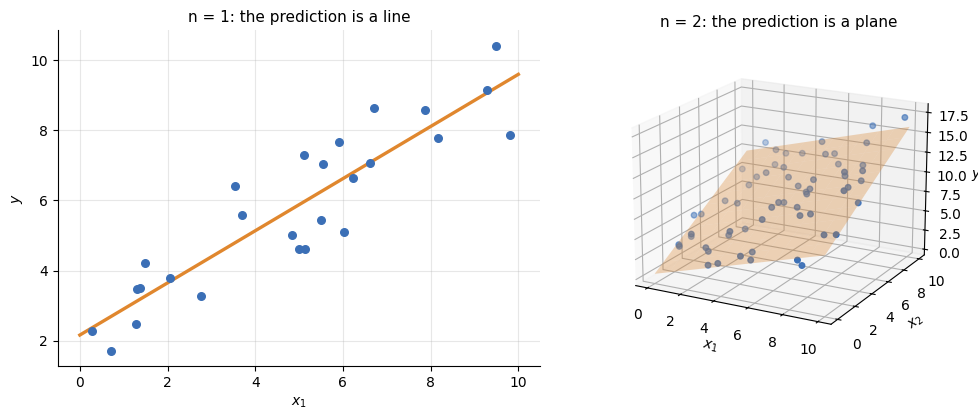
With one feature the model draws a line through the data, with two a plane, and beyond that a hyperplane that can no longer be drawn.
4.2 The problem to solve
Given the training set \(\{(x^{(i)}, y^{(i)})\}_{i=1}^{m}\), ideally we would have \(h_\theta(x^{(i)}) = y^{(i)}\) at every point. Real targets are noisy (measurement error, unmodelled factors), so no line passes through them all, and the goal becomes to make the smallest total error. Least squares takes the squared residual as the error and sums it over the training set:
\[\boxed{ \theta^{*} = \arg\min_\theta \; \sum_{i=1}^{m}\left(\theta^T x^{(i)} - y^{(i)}\right)^2 }\]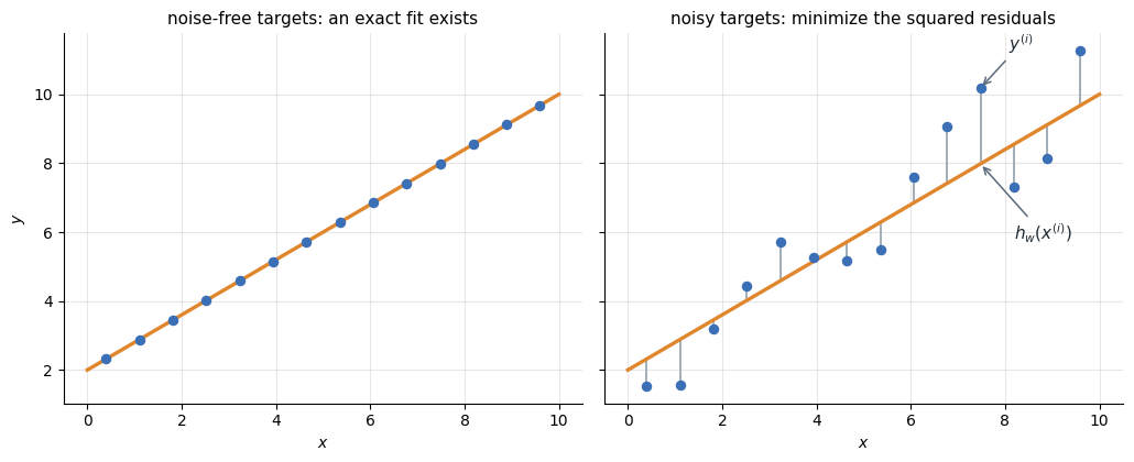
Left: if the targets were noise-free, the model could pass through every point. Right: real targets scatter around the trend, so each point leaves a residual between \(y^{(i)}\) and the prediction \(h_\theta(x^{(i)})\), and the fit minimizes their sum of squares (grey segments).
Remark: why the square rather than, say, the absolute value? Because this choice is provably optimal when the noise is Gaussian, a classic interview question that the next section unpacks.
4.3 Maximum likelihood: least squares justified
Give the data a generative story, using the estimation principle of Probabilistic formulation: each target is the linear prediction plus independent Gaussian noise,
\[\boxed{ y^{(i)} = \theta^T x^{(i)} + \varepsilon^{(i)}, \quad \varepsilon^{(i)} \sim \mathcal{N}(0, \sigma^2) }\]so \(p(y^{(i)} \mid x^{(i)}; \theta) = \mathcal{N}(\theta^T x^{(i)}, \sigma^2)\). The log-likelihood of the \(m\) i.i.d. examples separates into a constant and the sum of squares:
\[\ell(\theta) = \sum_{i=1}^{m} \log \mathcal{N}\!\left(y^{(i)} \mid \theta^T x^{(i)}, \sigma^2\right) = -\frac{m}{2}\log(2\pi\sigma^2) \;-\; \frac{1}{2\sigma^2}\sum_{i=1}^{m}\left(y^{(i)} - \theta^T x^{(i)}\right)^2\]Neither the constant nor the positive factor \(\tfrac{1}{2\sigma^2}\) moves the argmax, so:
\[\boxed{ \arg\max_\theta \; \ell(\theta) = \arg\min_\theta \; \sum_{i=1}^{m}\left(y^{(i)} - \theta^T x^{(i)}\right)^2 }\]Remark: this equivalence is the most important fact of the module. Least squares is not a convenient convention, it is the maximum-likelihood estimate under Gaussian noise.
The maximizer has a closed form. Writing the objective with the design matrix \(X\) and setting the gradient to zero,
\[\nabla_\theta\, \lVert X\theta - y \rVert^2 = 2\,X^T(X\theta - y) = 0\] \[\boxed{ \theta_{\mathrm{MLE}} = (X^T X)^{-1}X^T y }\]the normal equation, one matrix solve away from the data.
4.4 Maximum a posteriori: ridge regression
Maximum likelihood can overfit, especially when the model is flexible. The maximum a posteriori estimate maximizes the posterior instead, which by Bayes' rule is the likelihood times a prior on the parameters, here a zero-mean Gaussian:
\[\theta_{\mathrm{MAP}} = \arg\max_\theta \; p(y \mid X, \theta)\, p(\theta), \qquad \theta \sim \mathcal{N}(0, \tau^2 I)\]Taking logarithms adds \(-\lVert \theta \rVert^2 / 2\tau^2\) to the log-likelihood, and dropping the constants leaves a penalized least squares:
\[\boxed{ \theta_{\mathrm{MAP}} = \arg\min_\theta \; \sum_{i=1}^{m}\left(y^{(i)} - \theta^T x^{(i)}\right)^2 + \lambda \lVert \theta \rVert_2^2, \quad \lambda = \frac{\sigma^2}{\tau^2} }\]with, by the same zero-gradient computation, the closed form:
\[\boxed{ \theta_{\mathrm{MAP}} = (X^T X + \lambda I)^{-1}X^T y }\]This is ridge regression, and the penalty is often called weight decay. The Gaussian prior became the L2 penalty of General concepts, exactly the prior-to-penalty link of Probabilistic formulation.
Remark: \(\lambda \to 0\) recovers maximum likelihood, and a growing \(\lambda\) shrinks \(\theta\) toward zero and fights overfitting. A stronger prior (small \(\tau\)) means a larger \(\lambda\). Note also that \(X^T X + \lambda I\) is always invertible for \(\lambda > 0\), which rescues least squares exactly where it breaks down: strongly correlated features, or more features than examples.
4.5 The lasso: a penalty that selects
The ridge penalty came from a Gaussian prior. A Laplace prior yields the L1 penalty instead, the link noted in Probabilistic formulation:
\[\boxed{ \theta_{\mathrm{lasso}} = \arg\min_\theta \; \sum_{i=1}^{m}\left(y^{(i)} - \theta^T x^{(i)}\right)^2 + \lambda \lVert \theta \rVert_1 }\]The change looks small and its consequence is large: the lasso drives some coefficients to exactly zero, so it selects variables while it fits. Unlike ridge it has no closed form (the penalty is not differentiable at zero), so it is fitted by convex solvers. The reason for the selection is geometric. The constraint region \(\lVert \theta \rVert_1 \le t\) is a diamond with corners on the axes, and the elliptical contours of the squared error tend to touch it first at a corner, where a coordinate is zero. The rounded L2 ball has no corners, so ridge shrinks every coefficient smoothly but never zeroes one: ridge stabilizes, the lasso selects.

The rounded L2 ball is touched off the axes, keeping every coefficient nonzero, while the L1 diamond is touched at a corner, setting a coefficient to exactly zero.
As \(\lambda\) grows, more coefficients cross to zero, tracing the regularization path from the full model down to the empty one.

Each coefficient shrinks as \(\lambda\) increases and then hits exactly zero, so the lasso yields a compact, interpretable subset of regressors.
Remark: the elastic net blends the two penalties, \(\lambda\left(\alpha \lVert \theta \rVert_1 + (1-\alpha)\lVert \theta \rVert_2^2\right)\), keeping the lasso's selection with the ridge's stability under correlated features. As always, \(\lambda\) is chosen by the cross-validation of General concepts, often taking the largest \(\lambda\) within one standard error of the best for a simpler model.
Remark: prediction is not inference. Selecting variables with the lasso and then reporting textbook standard errors on the same data is invalid, the winner's curse again: the intervals ignore that the data already chose the variables. Honest inference needs sample splitting or a debiased estimator, the doorway to causal machine learning.
4.6 Basis functions: nonlinear in \(x\), linear in \(\theta\)
A straight line is often too rigid: the underfitting of General concepts appeared precisely when a low-capacity model met a curved trend. The fix is not to abandon the linear machinery but to project the input into a larger space, where the relationship is linear:
\[\boxed{ h_\theta(x) = \theta^T \phi(x) = \sum_{j=0}^{M-1} \theta_j\, \phi_j(x), \qquad \phi_0(x) = 1 }\]The \(\phi_j\) are basis functions, fixed before training. With \(\phi(x) = (1, x, x^2, \dots, x^d)\) they give polynomial regression, the running example of General concepts, and the identity \(\phi(x) = x\) recovers everything above. The model can now be wildly nonlinear in \(x\) yet stays linear in \(\theta\), so nothing changes in the fit: stack the \(\phi(x^{(i)})^T\) as the rows of the design matrix \(\Phi \in \mathbb{R}^{m \times M}\) and the two closed forms return verbatim:
\[\boxed{ \theta_{\mathrm{MLE}} = (\Phi^T \Phi)^{-1}\Phi^T y, \qquad \theta_{\mathrm{MAP}} = (\Phi^T \Phi + \lambda I)^{-1}\Phi^T y }\]Remark: the basis (its family and its size \(M\)) is a hyperparameter, chosen before training, while \(\theta\) is learned. Choosing \(M\) and \(\lambda\) is the model-selection problem settled by the cross-validation of General concepts.
4.7 Multiple outputs
Nothing restricts the target to a single number. To predict \(K\) values at once (say a house's price, heating cost, and property tax from the same features), let \(y^{(i)} \in \mathbb{R}^K\) and give each output its own parameter column, gathered in a matrix \(W \in \mathbb{R}^{M \times K}\):
\[\boxed{ h_W(x) = W^T \phi(x) \in \mathbb{R}^{K} }\]Stacking the targets as the rows of \(Y \in \mathbb{R}^{m \times K}\), the same derivations give the same closed forms, now solving all \(K\) regressions at once:
\[\boxed{ W_{\mathrm{MLE}} = (\Phi^T \Phi)^{-1}\Phi^T Y, \qquad W_{\mathrm{MAP}} = (\Phi^T \Phi + \lambda I)^{-1}\Phi^T Y }\]Remark: the expensive factor \((\Phi^T \Phi)^{-1}\) does not depend on the targets, so it is computed once and shared by all \(K\) outputs.
4.8 Summary
| Formula | |
|---|---|
| Model | \(h_\theta(x) = \theta^T \phi(x)\) |
| Maximum likelihood (least squares) | \(\theta_{\mathrm{MLE}} = (\Phi^T \Phi)^{-1}\Phi^T y\) |
| Maximum a posteriori (ridge) | \(\theta_{\mathrm{MAP}} = (\Phi^T \Phi + \lambda I)^{-1}\Phi^T y\) |
| Parameters, learned | \(\theta\) (or \(W\) for \(K\) outputs) |
| Hyperparameters, chosen by validation | the basis \(\phi\) and its size \(M\), the penalty \(\lambda\) |
The same linear score, passed through a squashing function instead of read directly, turns regression into classification, the subject of the next module.
Next: Linear classification · Course overview