
1. Introduction
Machine learning builds models that learn patterns from data instead of being explicitly programmed with rules. This module fixes the notation used throughout the course and maps the landscape of problems and models, so later modules can stay terse and formula-first.
Objectives
- Distinguish supervised, unsupervised, and reinforcement learning by their feedback signal.
- Situate the stages of a machine learning project and its feedback loops.
- Fix the notation used across the whole course.
- Define the training set, the hypothesis, and the design matrix.
- Adopt the intercept convention \(x_0 = 1\).
- Classify a supervised problem by the type of its output.
- Distinguish discriminative from generative models.
1.1 Types of learning
Machine learning problems are usually sorted into three paradigms. What separates them is not the algorithm but the feedback available during training: a label for every example, no labels at all, or a reward that arrives through interaction.
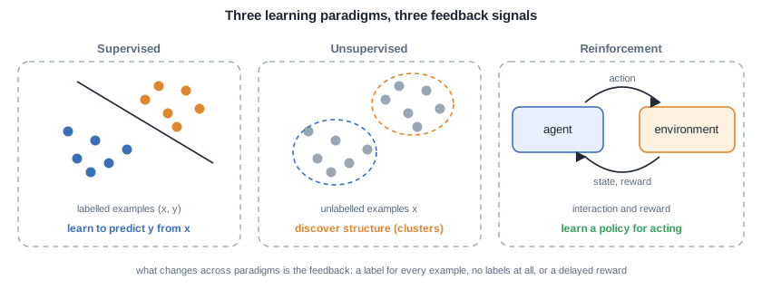
Supervised learning fits a mapping from labelled examples, unsupervised learning finds structure in unlabelled data, and reinforcement learning improves a policy through interaction with an environment.
Supervised learning. Each training example pairs an input \(x\) with the answer \(y\) the model should produce, and the goal is a mapping \(x \mapsto y\) that generalizes to inputs never seen in training. Predicting the price of a house from its features (regression) and deciding whether an email is spam (classification) are the canonical tasks. Labels make the objective explicit and progress measurable, which is why the theory is most developed here. Almost all of this course lives in this setting.
Unsupervised learning. Only the inputs \(x\) are available, and no label says what the right answer is. The goal shifts from prediction to description: group similar customers into segments (clustering), compress many correlated features into a few informative directions (dimensionality reduction), or estimate which regions of the input space are likely (density estimation). Success is harder to quantify, because there is no ground truth to compare against.
Reinforcement learning. There is no fixed dataset at all. An agent takes an action, the environment returns a new state and a reward, and the reward may arrive long after the action that earned it. The goal is a policy, a rule for choosing actions that maximizes the cumulative reward. Game playing and robotics are the typical examples. It is a field of its own and sits outside the scope of this course.
| Paradigm | Data | Feedback signal | What is learned | Canonical tasks |
|---|---|---|---|---|
| Supervised | pairs \((x, y)\) | the label \(y\) | a mapping \(h : x \mapsto y\) | regression, classification |
| Unsupervised | inputs \(x\) only | none | structure in the data | clustering, dimensionality reduction |
| Reinforcement | interaction | reward, often delayed | a policy for acting | control, game playing |
Remark: the boundaries are not rigid. Semi-supervised learning mixes a few labelled examples with many unlabelled ones, and self-supervised learning manufactures labels from the data itself, for example by hiding a word and predicting it. Both reuse the supervised machinery introduced in this course.
1.2 The workflow
A machine learning project is not a straight line from data to model. It runs as a loop: every evaluation reveals something that sends the work back to an earlier stage, and once deployed, a model faces new data that eventually restarts the cycle.

The solid path is the nominal order. The dashed arrows are where real projects spend most of their time: reworking features and models after evaluation, and retraining after monitoring.
- Define the problem and gather data. Turn the question into a prediction task by fixing the input \(x\), the target \(y\), and the metric that counts as success. The choices made here bound everything downstream, because no model can recover information the data does not contain.
- Explore and preprocess the data. Inspect distributions, missing values, and outliers, then clean, encode, and scale the features. Set aside a test set before tuning anything against it, so the final performance estimate stays honest.
- Train candidate models. Start with a simple baseline, then fit richer families by minimizing a loss over the parameters \(\theta\) (General concepts).
- Evaluate and compare. Measure each candidate on data it has never seen, with validation and cross-validation (General concepts) and a metric matched to the problem. The verdict usually points back to step 2 or 3: better features, another model family, or more data.
- Deploy and monitor. In production the incoming data drifts away from the training distribution, so performance must be watched and retraining planned. That discipline has its own course: MLOps.
Remark: in practice most of the effort goes into steps 1, 2, and 4. Training itself is often the cheapest step, and the ceiling on model quality is set by the data.
1.3 Notation and setup
1.3.1 Training set
The training set is defined as a collection of \(m\) labelled examples:
\[\boxed{ \{(x^{(i)}, y^{(i)})\}_{i=1}^{m} }\]Symbols:
- \(x^{(i)}\) is the input (feature vector) of the \(i\)-th example.
- \(y^{(i)}\) is its target (label).
- \(m\) is the number of training examples.
- \(n\) is the number of features.
- \(x_j^{(i)}\) is the \(j\)-th feature of the \(i\)-th example.
Remark: the superscript \((i)\) indexes the example and the subscript \(j\) indexes the feature, so \(x_j^{(i)}\) is feature \(j\) of example \(i\).
By convention the input is augmented with a constant intercept term \(x_0 = 1\), so \(x \in \mathbb{R}^{n+1}\) and the parameters are \(\theta \in \mathbb{R}^{n+1}\).
\[\boxed{ x_0 = 1, \quad x \in \mathbb{R}^{n+1}, \quad \theta \in \mathbb{R}^{n+1} }\]Remark: the intercept lets a single dot product \(\theta^T x\) carry the bias term, so no separate constant has to be written.
1.3.2 Hypothesis
A hypothesis is defined as a function chosen from a model family that maps an input to a prediction:
\[\boxed{ h_\theta : x \mapsto h_\theta(x) }\]Learning is the search, over the parameters \(\theta\), for the hypothesis that best fits the training set.
1.3.3 Design matrix
The design matrix stacks the \(m\) transposed inputs row by row, and the target vector collects the labels:
\[\boxed{ X = \begin{bmatrix} (x^{(1)})^{T} \\ \vdots \\ (x^{(m)})^{T} \end{bmatrix}, \quad y = \begin{bmatrix} y^{(1)} \\ \vdots \\ y^{(m)} \end{bmatrix} }\]Here \(X \in \mathbb{R}^{m \times (n+1)}\) (each augmented input is a row) and \(y \in \mathbb{R}^{m}\).
Remark: with this layout many models reduce to compact matrix expressions, for example a linear prediction over all examples is \(X\theta\).
1.4 Types of problems and models
1.4.1 Type of prediction
A supervised problem is named by the nature of its target \(y\).
| Type | Target | Goal |
|---|---|---|
| Regression | \(y \in \mathbb{R}\) | predict a continuous value |
| Classification | \(y \in \{1, \dots, k\}\) | predict one of \(k\) discrete classes |
Remark: binary classification is the case \(k = 2\), often coded as \(y \in \{0, 1\}\) or \(y \in \{-1, +1\}\).
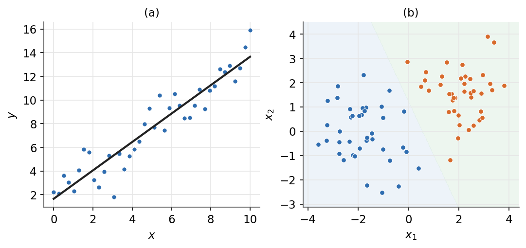
Left: regression fits a continuous output. Right: classification separates the input space into classes.
1.4.2 Type of model
A model is discriminative if it learns the conditional \(p(y \mid x)\) directly, and generative if it models how the data are generated, \(p(x \mid y)\) and \(p(y)\), then inverts via Bayes' rule:
\[\boxed{ p(y \mid x) = \frac{p(x \mid y)\, p(y)}{p(x)} }\]| Aspect | Discriminative | Generative |
|---|---|---|
| Goal | model the boundary between classes | model how each class generates data |
| What is learned | \(p(y \mid x)\) directly | \(p(x \mid y)\) and \(p(y)\), then Bayes |
| Examples | logistic regression, SVM | Gaussian discriminant analysis, naive Bayes |
Remark: \(p(x)\) is the same for every class, so for classification it can be dropped and the most probable class taken via \(\arg\max_y\, p(x \mid y)\, p(y)\).
1.4.3 Putting it together
The output type fixes regression vs classification, and the modelling choice fixes discriminative vs generative. Together they select a model family.
graph TD
  A["supervised problem"] --> B{"output type?"}
  B -->|"continuous"| C["regression"]
  B -->|"discrete"| D["classification"]
  D --> E{"model type?"}
  E -->|"discriminative"| F["logistic regression, SVM"]
  E -->|"generative"| G["GDA, naive Bayes"]
With the problem framed and the notation fixed, the next part turns to what learning really demands: minimizing a loss is easy, generalizing beyond the training set is the challenge.
Next: General concepts · Course overview