
1. Introduction
This course continues directly from the Machine Learning course, which closed the Linear classification part with a key remark: a perceptron is a single unit, and stacked into layers it becomes a neural network. This lesson makes that bridge explicit. It recalls what one unit can do, shows the concrete task (XOR) where a single unit fails, and fixes the notation used throughout the rest of the course.
Objectives
- Recall the perceptron as a single unit with a step activation and a linear boundary.
- See why one unit cannot solve XOR, motivating hidden layers.
- Understand what "deep" means and why hidden layers learn features.
- Adopt the explicit-bias, per-layer notation used across this course.
- Read a network as a composition of layer maps from input to prediction.
1.1 The perceptron, recalled
The perceptron from the Machine Learning course is a single computational unit. It scores an input with a linear combination of its features and passes that score through a hard threshold. With parameters \(w\) and the step activation \(g\), its hypothesis is:
\[\boxed{ h(x) = g(w^T x), \quad g(z) = \begin{cases} 1 & \text{if } z \ge 0 \\ 0 & \text{otherwise} \end{cases} }\]The equation \(w^T x = 0\) is a hyperplane, so the perceptron splits the input space with a single flat boundary. Points on one side are labelled \(1\), points on the other are labelled \(0\).
Remark: the boundary is linear because the score \(w^T x\) is linear in \(x\). The threshold only chooses a side, it does not bend the boundary.
1.2 Why one unit is not enough
A single linear boundary can only solve problems whose classes are linearly separable, that is, separable by one straight cut. Many simple problems are, but not all. The classic counterexample is the exclusive-or (XOR) function of two binary inputs.
The truth tables below compare AND, OR, and XOR:
| \(x_1\) | \(x_2\) | AND | OR | XOR |
|---|---|---|---|---|
| 0 | 0 | 0 | 0 | 0 |
| 0 | 1 | 0 | 1 | 1 |
| 1 | 0 | 0 | 1 | 1 |
| 1 | 1 | 1 | 1 | 0 |
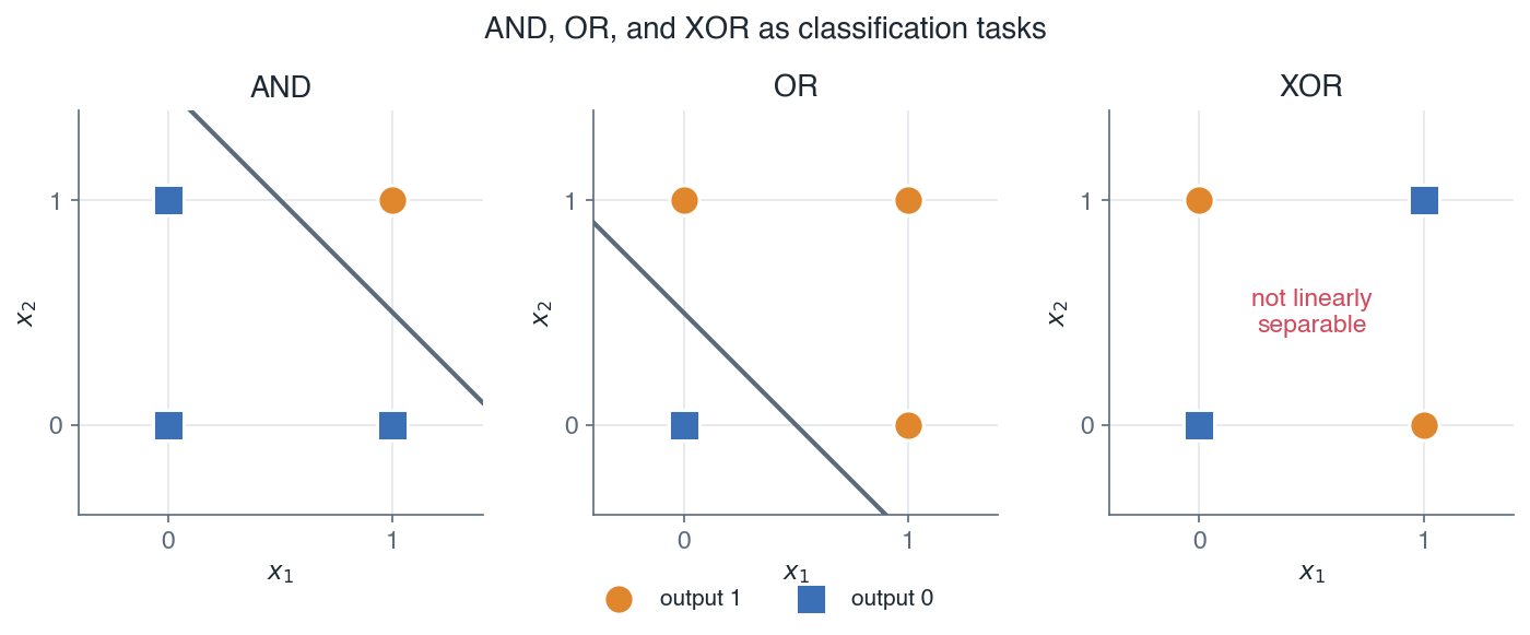
AND and OR are separable by a single straight line, but XOR is not, which is why one unit cannot solve it.
For AND and OR the two output classes can be separated by a single line, so a perceptron solves them. For XOR the positive points \((0,1)\) and \((1,0)\) sit on one diagonal and the negative points \((0,0)\) and \((1,1)\) sit on the other. No single straight line can separate them.
Remark: XOR is not a special curiosity. It shows that some patterns are inherently nonlinear, so any model built from one linear boundary is fundamentally limited. The fix is to combine several units.
If we place a layer of units between the input and the output, the first units can carve the space with several boundaries and a later unit can combine their outputs. Two lines can isolate the XOR pattern where one cannot. That intermediate layer is a hidden layer, and it is what turns a single unit into a network.
1.3 From units to networks
Stacking units into layers, and layers into a pipeline, gives a neural network. A network is deep when it has more than one hidden layer between the input and the output. Each layer applies a linear map followed by a nonlinear activation, and the layers are composed so the output of one feeds the input of the next.
The payoff is representation learning. In classical machine learning we hand-craft features, then feed them to a linear model. In a deep network the hidden layers learn their own features from raw input: early layers capture simple patterns and later layers combine them into more abstract ones. We specify the architecture and the objective, and the network discovers the intermediate representations by training.
Remark: stacking linear maps alone would collapse back to a single linear map, so the nonlinear activation \(g\) between layers is essential. Without it, no depth would add expressive power. Activation functions are covered in the next lessons.
1.4 Notation for this course
The Machine Learning course folded the bias into the score with the intercept convention \(x_0 = 1\), so a single dot product \(w^T x\) carried the constant term. This course keeps the bias explicit and uses a separate weight matrix per layer. This is the seam between the two courses: from here on, no augmented input and no folded bias.
1.4.1 A single unit
With explicit bias, one unit has a weight vector \(w\) and a scalar bias \(b\). Its activation is:
\[\boxed{ a = g(w^T x + b) }\]The score \(w^T x + b\) is the same affine function as before, only now the bias \(b\) is written out instead of hidden inside \(w\).
1.4.2 A layer and a network
Group the units of layer \(l\) into a weight matrix \(W^{[l]}\) and a bias vector \(b^{[l]}\). The layer computes a pre-activation \(z^{[l]}\), then an activation \(a^{[l]}\):
\[\boxed{ z^{[l]} = W^{[l]} a^{[l-1]} + b^{[l]}, \quad a^{[l]} = g^{[l]}(z^{[l]}) }\]The input feeds the first layer as \(a^{[0]} = x\), and for an \(L\)-layer network the prediction is the last activation:
\[\boxed{ a^{[0]} = x, \quad \hat{y} = a^{[L]} }\]So the network is a composition of layer maps: \(x = a^{[0]} \mapsto a^{[1]} \mapsto \cdots \mapsto a^{[L]} = \hat{y}\).
1.4.3 Symbol table
| Symbol | Meaning | Shape |
|---|---|---|
| \(L\) | number of layers | scalar |
| \(n_l\) | number of units in layer \(l\) | scalar |
| \(W^{[l]}\) | weight matrix of layer \(l\) | \(n_l \times n_{l-1}\) |
| \(b^{[l]}\) | bias vector of layer \(l\) | \(n_l\) |
| \(z^{[l]}\) | pre-activation of layer \(l\) | \(n_l\) |
| \(a^{[l]}\) | activation of layer \(l\) | \(n_l\) |
| \(g^{[l]}\) | activation function of layer \(l\) | applied elementwise |
| \(\hat{y}\) | prediction, equal to \(a^{[L]}\) | \(n_L\) |
Remark: the activation \(g^{[l]}\) acts componentwise, so an elementwise product later on is written with the Hadamard symbol \(\odot\). The superscript in brackets, \([l]\), indexes the layer, not an exponent.
The following diagram shows the smallest useful network: an input layer, one hidden layer, and an output layer.
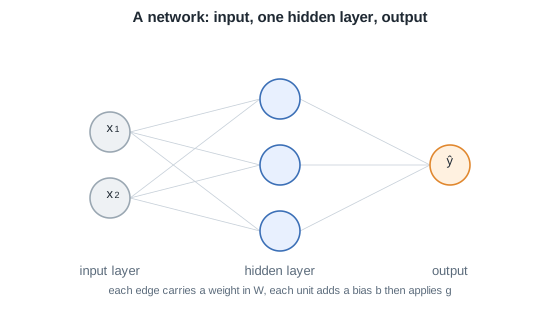
A neural network: an input layer, one hidden layer, and an output. Each edge carries a weight and each unit adds a bias then applies an activation g.
Each arrow carries a weight from \(W^{[l]}\), and every hidden and output unit adds its bias from \(b^{[l]}\) before applying its activation. This two-unit hidden layer is exactly what lets the network solve XOR, the task that defeated a single unit.
The next lesson formalizes this picture as the multilayer perceptron, writing the full forward pass layer by layer and choosing the activation functions.
Next: Multilayer perceptron · Course overview