
7. Decision trees and ensemble methods
Why trust one model when a committee can vote? This module builds the ensemble toolbox: the bootstrap and bagging to cut variance, AdaBoost to turn weak learners into a strong one, decision trees as the base learner of choice, and random forests as the combination that wins in practice.
7.1 Why a single model?
Every module so far trains one model and keeps it. A committee of \(M\) models is almost always better than any single member. The combination is an average for regression and a majority vote for classification:
\[\boxed{ h_{\text{com}}(x) = \frac{1}{M}\sum_{i=1}^{M} h_i(x) \ \ \text{(regression)}, \qquad h_{\text{com}}(x) = \text{majority vote over } h_1(x), \dots, h_M(x) \ \ \text{(classification)} }\]The members can come from \(M\) different algorithms, from one algorithm run with \(M\) hyperparameter settings, or, most interestingly, from one identical algorithm trained \(M\) times. Two families dominate that last case, and they are complementary:
| Family | Base models | Built | Mainly cuts |
|---|---|---|---|
| Bagging | high capacity (deep trees) | in parallel, on resampled data | variance |
| Boosting | low capacity (stumps) | sequentially, on reweighted data | bias |
7.2 The bootstrap: averaging away variance
Why does combining help? Train the same flexible model, a degree-25 polynomial, on 100 different training sets and the individual fits disagree wildly. Their average, however, hugs the true curve.
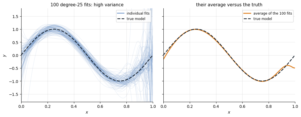
Left: 100 degree-25 fits, one per training set, each chasing its own noise. Right: their average is far closer to the truth, the fluctuations cancel.
The gain is quantifiable. If \(B\) models each have variance \(\sigma^2\) and pairwise correlation \(\rho\), the variance of their average is
\[\boxed{ \rho\sigma^2+\frac{1-\rho}{B}\,\sigma^2 }\]For independent models (\(\rho = 0\)) the variance shrinks like \(\sigma^2/B\). The catch: this needs many training sets, and outside of synthetic data we have exactly one. The bootstrap manufactures more by resampling the one we have, drawing \(N\) examples with replacement:
\[\boxed{ D_{\text{boot}} = \left\{ \left(x^{(i_1)}, y^{(i_1)}\right), \dots, \left(x^{(i_N)}, y^{(i_N)}\right) \right\}, \qquad i_k \ \text{drawn uniformly from} \ \{1, \dots, N\} }\]The same example can appear several times in one resample, and the probability that a given example never appears is \((1-\tfrac1N)^N\to e^{-1}\approx0.37\): about 37% of the data is left out of each resample. These are its out-of-bag (OOB) examples, which random forests will put to work below.
7.3 Bagging
Bagging (Bootstrap AGGregating) is the committee built from the bootstrap: resample \(m\) training sets, train one model on each, combine the votes.
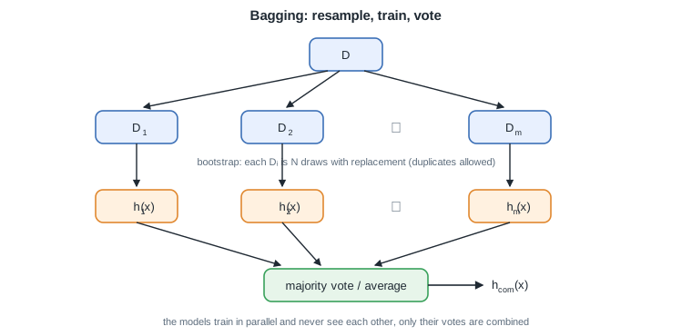
One dataset becomes \(m\) bootstrap resamples, each trains its own model, and only the votes meet.
\[\boxed{ h_{\text{bag}}(x)=\frac{1}{m}\sum_{i=1}^{m} h_i(x) \ \ \text{(regression)}, \qquad h_{\text{bag}}(x)=\mathrm{sign}\!\left(\sum_{i=1}^{m} h_i(x)\right) \ \ \text{(2 classes)}, \qquad \hat{y}=\arg\max_c \ \text{votes for } c \ \ \text{(K classes)} }\]Remark: averaging leaves bias unchanged while shrinking variance, so bagging suits base models with low bias and high variance, exactly the deep decision trees of section 8.5. A model that underfits stays underfitting after bagging.
7.4 Boosting: AdaBoost
Boosting takes the opposite bet: combine many weak learners, models barely better than chance, into a strong one. The ensemble is a weighted sum built one learner at a time:
\[\boxed{ H_T(x)=\sum_{t=1}^{T}\alpha_t\,h_t(x) }\]Three differences with bagging:
- The combination is weighted: an accurate learner earns a large vote \(\alpha_t\), a mediocre one a small vote.
- There is no bootstrap: every example is used to train every learner.
- The data is reweighted: examples misclassified by \(h_t\) gain weight, so \(h_{t+1}\) concentrates on them.
7.4.1 The algorithm
With labels \(y\in\{-1,+1\}\), keep one weight \(w^{(i)}\) per example, initialized to \(1/N\). At each round \(t = 1, \dots, T\):
- Train the weak learner \(h_t\) on the weighted data.
- Compute its weighted error \(\varepsilon_t = \sum_{i \in \mathcal{M}_t} w^{(i)}\) over the misclassified set \(\mathcal{M}_t\).
- Give it its vote, large when the error is small:
- Reweight and renormalize, so misclassified examples (\(y^{(i)}h_t(x^{(i)})<0\)) gain weight:
The final classifier is the weighted vote \(H_T(x) = \mathrm{sign}\big(\sum_t \alpha_t h_t(x)\big)\).
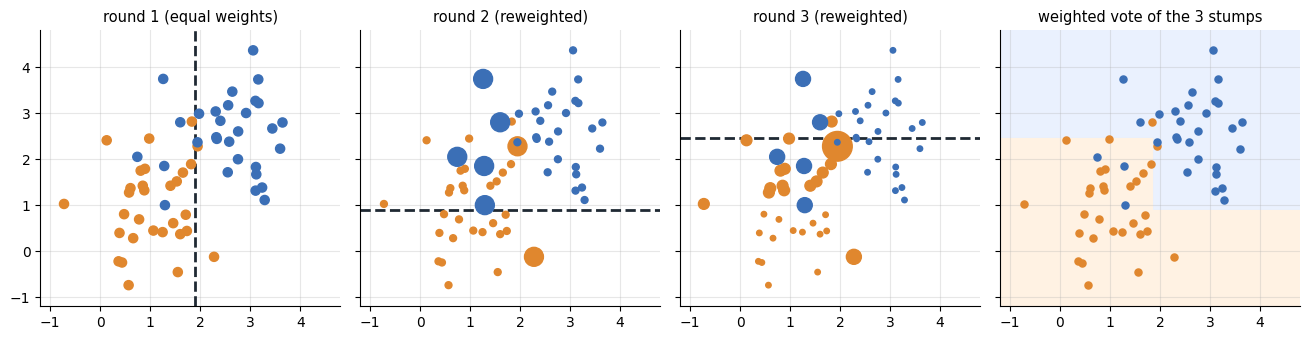
Each round fits one stump to the weighted data (dot size = weight). Misclassified points inflate, steering the next stump, and the weighted vote of three axis-aligned cuts already draws a jagged, nonlinear boundary.
Remark: the classic weak learner is the stump, a one-split tree perpendicular to an axis. Stumps are extremely fast, their combination gives the staircase boundaries above, and the learned \(\alpha_t\) double as a ranking of useful features: the features whose stumps earn large votes are the informative ones.
7.4.2 Gradient boosting
Gradient boosting generalizes the idea to any differentiable loss \(L\). At stage \(t\) it fits the next learner to the negative gradient of the loss evaluated at the current model, the pseudo-residual defined as
\[\boxed{ r^{(i)}_t=-\left[\frac{\partial L\big(y^{(i)},f(x^{(i)})\big)}{\partial f}\right]_{f=H_{t-1}} }\]The model is then updated with a learning rate (shrinkage) \(\nu\in(0,1]\):
\[\boxed{ H_t=H_{t-1}+\nu\,\alpha_t\,h_t }\]Remark: with squared-error loss the pseudo-residual is just the ordinary residual \(y^{(i)}-H_{t-1}(x^{(i)})\), so each tree fits what the current model still gets wrong.
| property | bagging | boosting |
|---|---|---|
| training | parallel, independent | sequential, each on the previous errors |
| base learners | deep, low bias | shallow, high bias |
| mainly reduces | variance | bias |
| reweighting | none (bootstrap) | weights or pseudo-residuals |
7.5 Decision trees
7.5.1 From stumps to trees
A stump asks one question about one feature. Chain the questions, each answer leading to the next stump, and you get a decision tree: a root, internal nodes, and leaves that tile the input space.
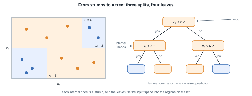
Three splits carve the plane into four regions (left), and the same three splits read as a tree (right): the root and internal nodes test features, the leaves predict.
7.5.2 Tree as a partition
A CART tree partitions the input space into \(M\) disjoint regions \(R_1,\dots,R_M\) (the leaves) and predicts a constant \(c_m\) on each. The prediction is defined as
\[\boxed{ h(x)=\sum_{m=1}^{M} c_m\,\mathbf{1}\{x\in R_m\} }\]Each internal node tests one feature against a threshold, \(x_j\le s\), sending an example left or right. A path from the root to a leaf is a conjunction of such tests.
Remark: the regions are axis-aligned boxes, so the decision boundary is a staircase. A single tree has low bias but high variance: left unchecked it keeps splitting until it isolates every outlier.
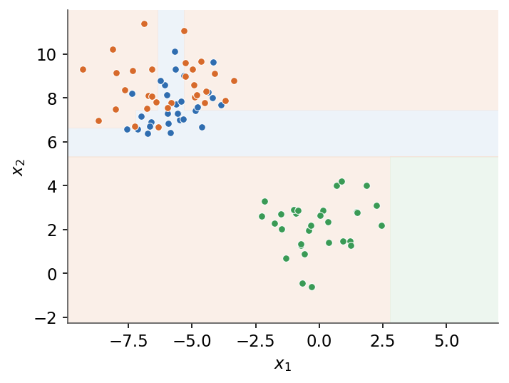
A tree carves the input space into axis-aligned regions, each with a constant prediction.
7.5.3 Impurity and split selection
Which question should a node ask? The one that leaves the children as pure as possible. For a region with class proportions \(\hat p_k\), impurity measures how mixed the labels are. The Gini index is defined as
\[\boxed{ G = 1-\sum_{k}\hat p_k^{\,2} }\]and the entropy as
\[\boxed{ H = -\sum_{k}\hat p_k\log_2\hat p_k }\]A candidate split sends \(N_-\) examples to child \(R_-\) and \(N_+\) to child \(R_+\) out of \(N\). Its information gain is defined as
\[\boxed{ IG = I(\text{parent})-\frac{N_-}{N}\,I(R_-)-\frac{N_+}{N}\,I(R_+) }\]where \(I\) is the chosen impurity. CART greedily picks the feature and threshold that maximize \(IG\) at each node, and a node whose impurity is already low is not worth splitting: that is the overfitting dial.
| criterion | formula | range (binary) | note |
|---|---|---|---|
| Gini | \(1-\sum_k\hat p_k^{2}\) | \([0,0.5]\) | cheaper, no logarithm |
| entropy | \(-\sum_k\hat p_k\log_2\hat p_k\) | \([0,1]\) | information-theoretic |
Remark: the two criteria almost always pick the same split. Gini is the default in most implementations because it avoids the logarithm.
7.5.4 Regression trees
For regression the leaf value is the mean of the targets in the region, defined as
\[\boxed{ c_m=\frac{1}{N_m}\sum_{x^{(i)}\in R_m} y^{(i)} }\]and splits minimize the within-region squared error instead of a classification impurity.
7.5.5 Pruning
An unpruned tree fits the training set exactly and overfits. Cost-complexity pruning trades fit against tree size \(|T|\) (the number of leaves) through a penalty \(\alpha\ge0\):
\[\boxed{ C_\alpha(T)=\sum_{m} N_m\,I(R_m)+\alpha\,|T| }\]
Increasing \(\alpha\) collapses the weakest splits, yielding a nested sequence of subtrees. The best \(\alpha\) is chosen by the cross-validation of General concepts.
7.6 Random forests
A random forest is bagging applied to deep trees, plus a second source of randomness. The variance formula of section 8.2 said the residual term \(\rho\sigma^2\) survives averaging, so the trees must be decorrelated: at each split only a random subset of \(m_{\text{try}}\) features is considered as split candidates. The usual choices are
\[\boxed{ m_{\text{try}}=\lfloor\sqrt{n}\,\rfloor\ \text{(classification)},\qquad m_{\text{try}}=\lfloor n/3\rfloor\ \text{(regression)} }\]Restricting the candidate features stops every tree from splitting on the same dominant feature, which makes the trees' errors as uncorrelated as possible and lowers \(\rho\).
Remark: OOB error averages each tree's error over only the examples that tree never saw (the 37% of section 8.2), giving a cross-validation-like estimate at no extra cost.
| property | bagging | random forest |
|---|---|---|
| resampling | bootstrap | bootstrap |
| split candidates | all \(n\) features | random \(m_{\text{try}}\) features |
| tree correlation \(\rho\) | higher | lower |
| variance reduction | moderate | stronger |
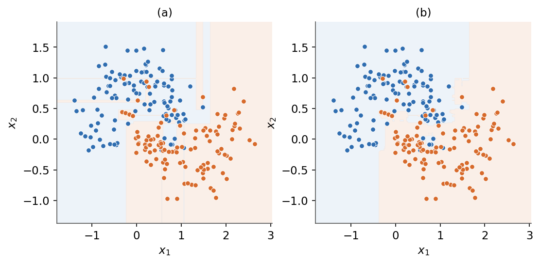
(a) A single deep tree overfits with a jagged boundary. (b) A random forest averages many trees for a smoother boundary.
This completes the supervised-learning core of the course. To take these models from a notebook to a running service, continue with the MLOps course.
Next: Course overview