
# 7. Decision trees and ensemble methods Why trust one model when a committee can vote? This module builds the ensemble toolbox: the bootstrap and bagging to cut variance, AdaBoost to turn weak learners into a strong one, decision trees as the base learner of choice, and random forests as the combination that wins in practice. ## 7.1 Why a single model? Every module so far trains one model and keeps it. A committee of $M$ models is almost always better than any single member. The combination is an average for regression and a majority vote for classification: $$\boxed{ h_{\text{com}}(x) = \frac{1}{M}\sum_{i=1}^{M} h_i(x) \ \ \text{(regression)}, \qquad h_{\text{com}}(x) = \text{majority vote over } h_1(x), \dots, h_M(x) \ \ \text{(classification)} }$$ The members can come from $M$ different algorithms, from one algorithm run with $M$ hyperparameter settings, or, most interestingly, from one identical algorithm trained $M$ times. Two families dominate that last case, and they are complementary: | Family | Base models | Built | Mainly cuts | | --- | --- | --- | --- | | Bagging | high capacity (deep trees) | in parallel, on resampled data | variance | | Boosting | low capacity (stumps) | sequentially, on reweighted data | bias | ## 7.2 The bootstrap: averaging away variance Why does combining help? Train the same flexible model, a degree-25 polynomial, on 100 different training sets and the individual fits disagree wildly. Their average, however, hugs the true curve. 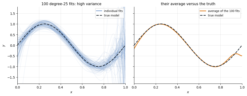 *Left: 100 degree-25 fits, one per training set, each chasing its own noise. Right: their average is far closer to the truth, the fluctuations cancel.* The gain is quantifiable. If $B$ models each have variance $\sigma^2$ and pairwise correlation $\rho$, the variance of their average is $$\boxed{ \rho\sigma^2+\frac{1-\rho}{B}\,\sigma^2 }$$ For independent models ($\rho = 0$) the variance shrinks like $\sigma^2/B$. The catch: this needs many training sets, and outside of synthetic data we have exactly one. The bootstrap manufactures more by resampling the one we have, drawing $N$ examples **with replacement**: $$\boxed{ D_{\text{boot}} = \left\{ \left(x^{(i_1)}, y^{(i_1)}\right), \dots, \left(x^{(i_N)}, y^{(i_N)}\right) \right\}, \qquad i_k \ \text{drawn uniformly from} \ \{1, \dots, N\} }$$ The same example can appear several times in one resample, and the probability that a given example never appears is $(1-\tfrac1N)^N\to e^{-1}\approx0.37$: about 37% of the data is left out of each resample. These are its out-of-bag (OOB) examples, which random forests will put to work below. ## 7.3 Bagging Bagging (Bootstrap AGGregating) is the committee built from the bootstrap: resample $m$ training sets, train one model on each, combine the votes. 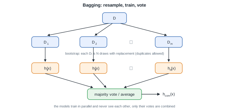 *One dataset becomes $m$ bootstrap resamples, each trains its own model, and only the votes meet.* $$\boxed{ h_{\text{bag}}(x)=\frac{1}{m}\sum_{i=1}^{m} h_i(x) \ \ \text{(regression)}, \qquad h_{\text{bag}}(x)=\mathrm{sign}\!\left(\sum_{i=1}^{m} h_i(x)\right) \ \ \text{(2 classes)}, \qquad \hat{y}=\arg\max_c \ \text{votes for } c \ \ \text{(K classes)} }$$ *Remark:* averaging leaves bias unchanged while shrinking variance, so bagging suits base models with low bias and high variance, exactly the deep decision trees of section 8.5. A model that underfits stays underfitting after bagging. ## 7.4 Boosting: AdaBoost Boosting takes the opposite bet: combine many weak learners, models barely better than chance, into a strong one. The ensemble is a weighted sum built one learner at a time: $$\boxed{ H_T(x)=\sum_{t=1}^{T}\alpha_t\,h_t(x) }$$ Three differences with bagging: 1. The combination is **weighted**: an accurate learner earns a large vote $\alpha_t$, a mediocre one a small vote. 2. There is **no bootstrap**: every example is used to train every learner. 3. The data is **reweighted**: examples misclassified by $h_t$ gain weight, so $h_{t+1}$ concentrates on them. ### 7.4.1 The algorithm With labels $y\in\{-1,+1\}$, keep one weight $w^{(i)}$ per example, initialized to $1/N$. At each round $t = 1, \dots, T$: 1. Train the weak learner $h_t$ on the weighted data. 2. Compute its weighted error $\varepsilon_t = \sum_{i \in \mathcal{M}_t} w^{(i)}$ over the misclassified set $\mathcal{M}_t$. 3. Give it its vote, large when the error is small: $$\boxed{ \alpha_t=\tfrac12\log\frac{1-\varepsilon_t}{\varepsilon_t} }$$ 4. Reweight and renormalize, so misclassified examples ($y^{(i)}h_t(x^{(i)})<0$) gain weight: $$\boxed{ w^{(i)}\leftarrow w^{(i)}\exp\!\big(-\alpha_t\,y^{(i)}h_t(x^{(i)})\big) }$$ The final classifier is the weighted vote $H_T(x) = \mathrm{sign}\big(\sum_t \alpha_t h_t(x)\big)$. 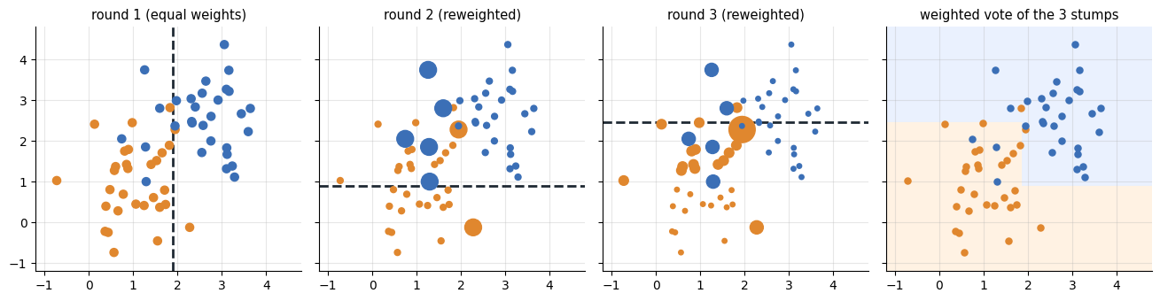 *Each round fits one stump to the weighted data (dot size = weight). Misclassified points inflate, steering the next stump, and the weighted vote of three axis-aligned cuts already draws a jagged, nonlinear boundary.* *Remark:* the classic weak learner is the stump, a one-split tree perpendicular to an axis. Stumps are extremely fast, their combination gives the staircase boundaries above, and the learned $\alpha_t$ double as a ranking of useful features: the features whose stumps earn large votes are the informative ones. ### 7.4.2 Gradient boosting Gradient boosting generalizes the idea to any differentiable loss $L$. At stage $t$ it fits the next learner to the negative gradient of the loss evaluated at the current model, the pseudo-residual defined as $$\boxed{ r^{(i)}_t=-\left[\frac{\partial L\big(y^{(i)},f(x^{(i)})\big)}{\partial f}\right]_{f=H_{t-1}} }$$ The model is then updated with a learning rate (shrinkage) $\nu\in(0,1]$: $$\boxed{ H_t=H_{t-1}+\nu\,\alpha_t\,h_t }$$ *Remark:* with squared-error loss the pseudo-residual is just the ordinary residual $y^{(i)}-H_{t-1}(x^{(i)})$, so each tree fits what the current model still gets wrong. | property | bagging | boosting | | --- | --- | --- | | training | parallel, independent | sequential, each on the previous errors | | base learners | deep, low bias | shallow, high bias | | mainly reduces | variance | bias | | reweighting | none (bootstrap) | weights or pseudo-residuals | ## 7.5 Decision trees ### 7.5.1 From stumps to trees A stump asks one question about one feature. Chain the questions, each answer leading to the next stump, and you get a decision tree: a root, internal nodes, and leaves that tile the input space. 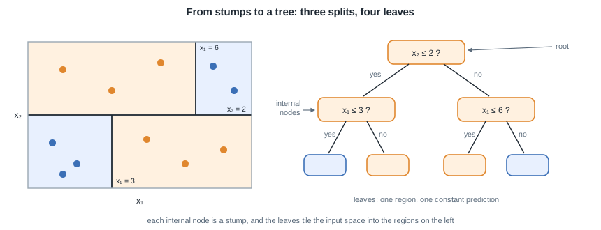 *Three splits carve the plane into four regions (left), and the same three splits read as a tree (right): the root and internal nodes test features, the leaves predict.* ### 7.5.2 Tree as a partition A CART tree partitions the input space into $M$ disjoint regions $R_1,\dots,R_M$ (the leaves) and predicts a constant $c_m$ on each. The prediction is defined as $$\boxed{ h(x)=\sum_{m=1}^{M} c_m\,\mathbf{1}\{x\in R_m\} }$$ Each internal node tests one feature against a threshold, $x_j\le s$, sending an example left or right. A path from the root to a leaf is a conjunction of such tests. *Remark:* the regions are axis-aligned boxes, so the decision boundary is a staircase. A single tree has low bias but high variance: left unchecked it keeps splitting until it isolates every outlier. 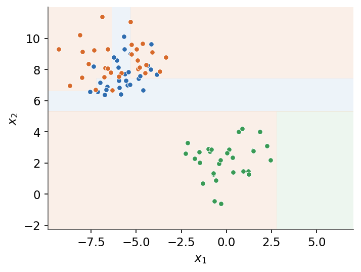 *A tree carves the input space into axis-aligned regions, each with a constant prediction.* ### 7.5.3 Impurity and split selection Which question should a node ask? The one that leaves the children as pure as possible. For a region with class proportions $\hat p_k$, impurity measures how mixed the labels are. The Gini index is defined as $$\boxed{ G = 1-\sum_{k}\hat p_k^{\,2} }$$ and the entropy as $$\boxed{ H = -\sum_{k}\hat p_k\log_2\hat p_k }$$ A candidate split sends $N_-$ examples to child $R_-$ and $N_+$ to child $R_+$ out of $N$. Its information gain is defined as $$\boxed{ IG = I(\text{parent})-\frac{N_-}{N}\,I(R_-)-\frac{N_+}{N}\,I(R_+) }$$ where $I$ is the chosen impurity. CART greedily picks the feature and threshold that maximize $IG$ at each node, and a node whose impurity is already low is not worth splitting: that is the overfitting dial. | criterion | formula | range (binary) | note | | --- | --- | --- | --- | | Gini | $1-\sum_k\hat p_k^{2}$ | $[0,0.5]$ | cheaper, no logarithm | | entropy | $-\sum_k\hat p_k\log_2\hat p_k$ | $[0,1]$ | information-theoretic | *Remark:* the two criteria almost always pick the same split. Gini is the default in most implementations because it avoids the logarithm. ### 7.5.4 Regression trees For regression the leaf value is the mean of the targets in the region, defined as $$\boxed{ c_m=\frac{1}{N_m}\sum_{x^{(i)}\in R_m} y^{(i)} }$$ and splits minimize the within-region squared error instead of a classification impurity. ### 7.5.5 Pruning An unpruned tree fits the training set exactly and overfits. Cost-complexity pruning trades fit against tree size $|T|$ (the number of leaves) through a penalty $\alpha\ge0$: $$\boxed{ C_\alpha(T)=\sum_{m} N_m\,I(R_m)+\alpha\,|T| }$$ Increasing $\alpha$ collapses the weakest splits, yielding a nested sequence of subtrees. The best $\alpha$ is chosen by the cross-validation of [General concepts](/en/Machine%20Learning/02%20General%20concepts). ## 7.6 Random forests A random forest is bagging applied to deep trees, plus a second source of randomness. The variance formula of section 8.2 said the residual term $\rho\sigma^2$ survives averaging, so the trees must be decorrelated: at each split only a random subset of $m_{\text{try}}$ features is considered as split candidates. The usual choices are $$\boxed{ m_{\text{try}}=\lfloor\sqrt{n}\,\rfloor\ \text{(classification)},\qquad m_{\text{try}}=\lfloor n/3\rfloor\ \text{(regression)} }$$ Restricting the candidate features stops every tree from splitting on the same dominant feature, which makes the trees' errors as uncorrelated as possible and lowers $\rho$. *Remark:* OOB error averages each tree's error over only the examples that tree never saw (the 37% of section 8.2), giving a cross-validation-like estimate at no extra cost. | property | bagging | random forest | | --- | --- | --- | | resampling | bootstrap | bootstrap | | split candidates | all $n$ features | random $m_{\text{try}}$ features | | tree correlation $\rho$ | higher | lower | | variance reduction | moderate | stronger | 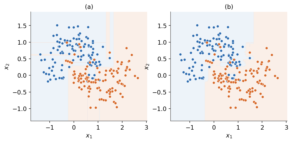 *(a) A single deep tree overfits with a jagged boundary. (b) A random forest averages many trees for a smoother boundary.* *This completes the supervised-learning core of the course. To take these models from a notebook to a running service, continue with the [MLOps](/en/MLOps) course.* --- Next: [Course overview](/en/Machine%20Learning)