
3. Probabilistic formulation
Probability is the language machine learning uses to handle uncertainty. This module sets out the rules for discrete and continuous variables, takes a first look at information theory, shows the Bayesian way of turning probabilities into decisions, and defines the two estimation principles the course returns to again and again: maximum likelihood and maximum a posteriori.
3.1 Probability, discrete and continuous
A random variable takes values with probabilities that are non-negative and sum or integrate to one. A discrete variable has a probability mass function, a continuous one a probability density function:
\[\boxed{ \sum_x p(x) = 1 \qquad \int p(x)\, dx = 1, \quad p(x) \ge 0 }\]For a continuous variable, probability attaches to intervals through an integral, \(P(a \le X \le b) = \int_a^b p(x)\, dx\), not to single points.
3.2 Joint, conditional, and Bayes
Two variables have a joint distribution \(p(x, y)\). Summing (or integrating) out one variable gives the marginal, the sum rule, and the joint factors into a conditional times a marginal, the product rule:
\[\boxed{ p(x) = \sum_y p(x, y) \qquad p(x, y) = p(y \mid x)\, p(x) }\]Rearranging the product rule both ways gives Bayes' rule, which flips a conditional:
\[\boxed{ p(y \mid x) = \frac{p(x \mid y)\, p(y)}{p(x)} }\]Two variables are independent when the joint is the product of the marginals, \(p(x, y) = p(x)\, p(y)\).
3.3 A little information theory
The entropy of a distribution measures its uncertainty, the average number of bits needed to describe an outcome:
\[\boxed{ H(X) = -\sum_x p(x)\log p(x) }\]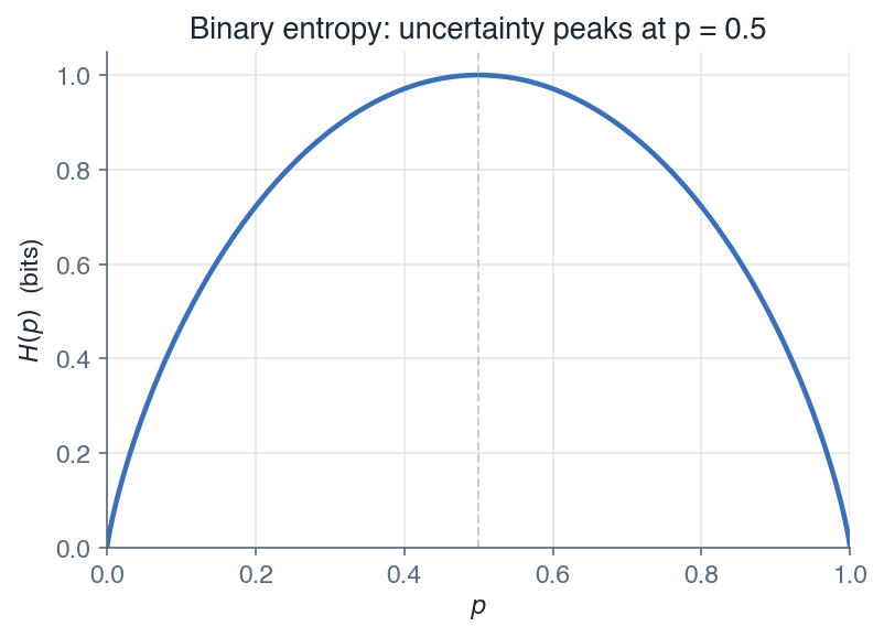
For a two-outcome variable the entropy is largest at \(p = 0.5\), where the outcome is hardest to predict, and zero when one outcome is certain.
The cross-entropy measures the cost of using a model \(q\) when the truth is \(p\), and the Kullback-Leibler divergence measures how far \(q\) sits from \(p\):
\[\boxed{ H(p, q) = -\sum_x p(x)\log q(x) \qquad D_{\mathrm{KL}}(p \,\|\, q) = \sum_x p(x)\log\frac{p(x)}{q(x)} \ge 0 }\]
Remark: minimizing the cross-entropy between the true labels and a model's predictions is the same as maximizing the likelihood of those labels. This is why classification networks minimize cross-entropy, a thread picked up in later modules.
3.4 Bayesian decision theory
To classify an input \(x\), the Bayesian rule uses the posterior over classes. Under the 0-1 loss, the decision that minimizes the expected loss is simply the most probable class, and because the posterior is proportional to the class-conditional density times the prior, it can be computed either way:
\[\boxed{ \hat{y} = \arg\max_y \; p(y \mid x) = \arg\max_y \; p(x \mid y)\, p(y) }\]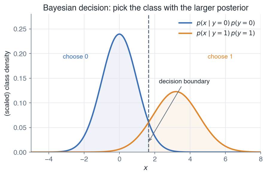
Each class contributes its density scaled by its prior, and the decision boundary falls where the two are equal. On each side the class with the larger posterior wins.
Remark: this is the optimal classifier, called the Bayes classifier. Every method later in the course is, in effect, an attempt to approximate these posteriors from data.
3.5 Maximum likelihood and maximum a posteriori
We rarely know the true distribution, so we estimate its parameters \(w\) from data. Maximum likelihood picks the \(w\) that makes the observed data most probable, usually maximized as a sum of log-likelihoods over the \(m\) examples:
\[\boxed{ w_{\mathrm{MLE}} = \arg\max_w \sum_{i=1}^{m} \log p(x^{(i)} \mid w) }\]In supervised learning the model parameterizes the conditional \(p(y \mid x; w)\), so the same principle applies to the conditional likelihood of the targets:
\[\boxed{ \ell(w) = \sum_{i=1}^{m} \log p\!\left(y^{(i)} \mid x^{(i)}; w\right) }\]Maximizing \(\ell\) is the same as minimizing the cost \(J(w) = -\ell(w)\), so the likelihood view and the cost-minimization view of General concepts are two faces of one objective.
Maximum a posteriori instead maximizes the posterior, which multiplies the likelihood by a prior on \(w\):
\[\boxed{ w_{\mathrm{MAP}} = \arg\max_w \; p(D \mid w)\, p(w) }\]Remark: maximum a posteriori is maximum likelihood plus a prior. A Gaussian prior on \(w\) becomes an L2 penalty and a Laplace prior an L1 penalty, which is exactly the regularization of the next module. With abundant data the prior washes out and the two estimators agree.
The next module turns these principles into a first concrete model: linear regression, where maximum likelihood and maximum a posteriori both land on closed-form fits.
Next: Linear regression · Course overview