
# 3. Probabilistic formulation Probability is the language machine learning uses to handle uncertainty. This module sets out the rules for discrete and continuous variables, takes a first look at information theory, shows the Bayesian way of turning probabilities into decisions, and defines the two estimation principles the course returns to again and again: maximum likelihood and maximum a posteriori. ## 3.1 Probability, discrete and continuous A random variable takes values with probabilities that are non-negative and sum or integrate to one. A discrete variable has a probability mass function, a continuous one a probability density function: $$\boxed{ \sum_x p(x) = 1 \qquad \int p(x)\, dx = 1, \quad p(x) \ge 0 }$$ For a continuous variable, probability attaches to intervals through an integral, $P(a \le X \le b) = \int_a^b p(x)\, dx$, not to single points. ## 3.2 Joint, conditional, and Bayes Two variables have a joint distribution $p(x, y)$. Summing (or integrating) out one variable gives the marginal, the sum rule, and the joint factors into a conditional times a marginal, the product rule: $$\boxed{ p(x) = \sum_y p(x, y) \qquad p(x, y) = p(y \mid x)\, p(x) }$$ Rearranging the product rule both ways gives Bayes' rule, which flips a conditional: $$\boxed{ p(y \mid x) = \frac{p(x \mid y)\, p(y)}{p(x)} }$$ Two variables are independent when the joint is the product of the marginals, $p(x, y) = p(x)\, p(y)$. ## 3.3 A little information theory The entropy of a distribution measures its uncertainty, the average number of bits needed to describe an outcome: $$\boxed{ H(X) = -\sum_x p(x)\log p(x) }$$ 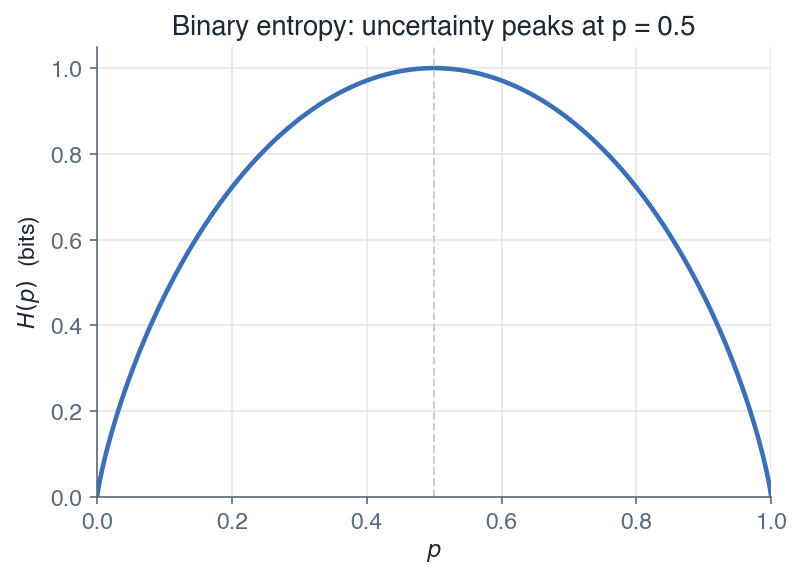 *For a two-outcome variable the entropy is largest at $p = 0.5$, where the outcome is hardest to predict, and zero when one outcome is certain.* The cross-entropy measures the cost of using a model $q$ when the truth is $p$, and the Kullback-Leibler divergence measures how far $q$ sits from $p$: $$\boxed{ H(p, q) = -\sum_x p(x)\log q(x) \qquad D_{\mathrm{KL}}(p \,\|\, q) = \sum_x p(x)\log\frac{p(x)}{q(x)} \ge 0 }$$ *Remark:* minimizing the cross-entropy between the true labels and a model's predictions is the same as maximizing the likelihood of those labels. This is why classification networks minimize cross-entropy, a thread picked up in later modules. ## 3.4 Bayesian decision theory To classify an input $x$, the Bayesian rule uses the posterior over classes. Under the 0-1 loss, the decision that minimizes the expected loss is simply the most probable class, and because the posterior is proportional to the class-conditional density times the prior, it can be computed either way: $$\boxed{ \hat{y} = \arg\max_y \; p(y \mid x) = \arg\max_y \; p(x \mid y)\, p(y) }$$ 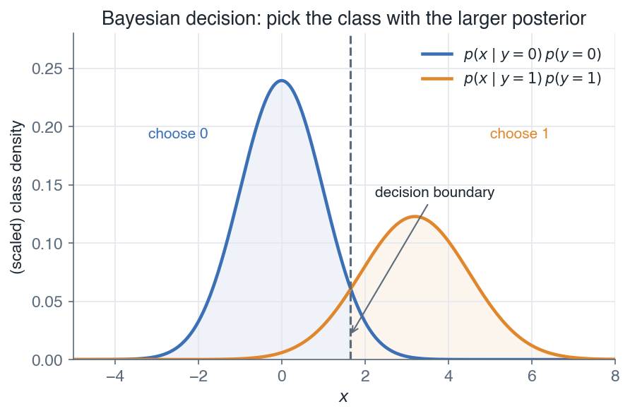 *Each class contributes its density scaled by its prior, and the decision boundary falls where the two are equal. On each side the class with the larger posterior wins.* *Remark:* this is the optimal classifier, called the Bayes classifier. Every method later in the course is, in effect, an attempt to approximate these posteriors from data. ## 3.5 Maximum likelihood and maximum a posteriori We rarely know the true distribution, so we estimate its parameters $w$ from data. Maximum likelihood picks the $w$ that makes the observed data most probable, usually maximized as a sum of log-likelihoods over the $m$ examples: $$\boxed{ w_{\mathrm{MLE}} = \arg\max_w \sum_{i=1}^{m} \log p(x^{(i)} \mid w) }$$ In supervised learning the model parameterizes the conditional $p(y \mid x; w)$, so the same principle applies to the conditional likelihood of the targets: $$\boxed{ \ell(w) = \sum_{i=1}^{m} \log p\!\left(y^{(i)} \mid x^{(i)}; w\right) }$$ Maximizing $\ell$ is the same as minimizing the cost $J(w) = -\ell(w)$, so the likelihood view and the cost-minimization view of [General concepts](/en/Machine%20Learning/02%20General%20concepts) are two faces of one objective. Maximum a posteriori instead maximizes the posterior, which multiplies the likelihood by a prior on $w$: $$\boxed{ w_{\mathrm{MAP}} = \arg\max_w \; p(D \mid w)\, p(w) }$$ *Remark:* maximum a posteriori is maximum likelihood plus a prior. A Gaussian prior on $w$ becomes an L2 penalty and a Laplace prior an L1 penalty, which is exactly the regularization of the next module. With abundant data the prior washes out and the two estimators agree. *The next module turns these principles into a first concrete model: linear regression, where maximum likelihood and maximum a posteriori both land on closed-form fits.* --- Next: [Linear regression](/en/Machine%20Learning/04%20Linear%20regression) · [Course overview](/en/Machine%20Learning)