
2. General concepts
The introduction fixed the notation and named the learning paradigms. Before fitting any particular model, this module covers what learning actually means. Making a model fit the data it has seen is easy, making it perform on data it has never seen is the whole game. Polynomial regression serves as the running example, and the module closes with the reason geometric intuition fails in high dimension.
2.1 Supervised versus unsupervised learning
The Introduction named the paradigms by their feedback signal. Formally, supervised learning starts from labelled pairs \(\{(x^{(i)}, y^{(i)})\}_{i=1}^{m}\) and searches a family of hypotheses for the \(h_w\) whose predictions sit closest to the targets, closeness being measured by a loss function. Unsupervised learning has only the inputs \(x^{(i)}\), so its objectives are built from the inputs alone: compact groups, informative directions, regions of high density.
Everything in this module is stated for the supervised case, which occupies the rest of the course. The questions it answers (how well does this model generalize, how complex should it be, how do I choose between candidates) arise unchanged in the unsupervised setting.
2.2 Minimizing a loss: polynomial regression
2.2.1 Loss function
A loss function \(L(z, y)\) is defined as a scalar penalty comparing a raw model score \(z\) (or a predicted probability \(\hat{y}\)) against the target \(y\). Smaller is better. Each family of models is characterized by its loss.
| Loss | Formula \(L(z,y)\) | Used by |
|---|---|---|
| Least squared error | \(\tfrac{1}{2}(y-z)^2\) | Linear regression |
| Logistic | \(\log\!\left(1+\exp(-yz)\right)\) | Logistic regression |
| Cross-entropy | \(-\left[\,y\log\hat{y}+(1-y)\log(1-\hat{y})\,\right]\) | Neural networks |
Remark: \(z\) denotes a raw score such as \(w^T x\), whereas \(\hat{y} \in (0,1)\) denotes a predicted probability, the model's estimate of the label \(y\). The cross-entropy row takes a probability \(\hat{y}\), not a raw score.
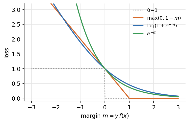
Margin-based losses, each a convex surrogate for the 0-1 loss that penalizes small or negative margins.
2.2.2 Cost function
The cost \(J(w)\) is defined as the sum of the per-example losses over the whole training set of \(m\) examples:
\[\boxed{\,J(w)=\sum_{i=1}^{m} L\!\left(h_w(x^{(i)}),\,y^{(i)}\right)\,}\]Training a model means choosing \(w\) to minimize \(J(w)\). The algorithms that carry out this minimization (closed forms, gradient descent) arrive with the model modules. This module asks a different question: what does a low value of \(J(w)\) actually prove?
Remark: the factor \(\tfrac{1}{2}\) in the squared error is a convention that cancels with the exponent when differentiating, leaving a clean gradient.
2.2.3 The running example: polynomial regression
To make everything concrete, take a single input \(x\) and fit a polynomial of degree \(d\) under the squared loss:
\[\boxed{ h_w(x) = w^T \phi(x) = \sum_{j=0}^{d} w_j\, x^{j}, \qquad \phi(x) = (1, x, x^2, \dots, x^d) }\]The model stays linear in \(w\), so least squares applies unchanged (the closed form is derived in Linear regression). The degree \(d\) is not fitted along with \(w\): it is fixed before fitting and decides how flexible the curve is allowed to be. A knob of that kind, chosen rather than learned, is called a hyperparameter, and \(d\) is our first one.
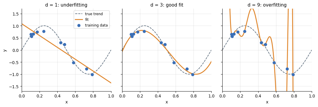
The same noisy sample fitted three ways. Degree 1 is too rigid to follow the trend, degree 3 captures it, and degree 9 weaves through every training point.
2.3 Training performance versus generalization
2.3.1 Generalization error
The quantity we care about is the generalization error, the expected loss on a fresh draw from the same population:
\[\boxed{ R(h) = \mathbb{E}_{(x, y)}\left[ L\!\left(h(x), y\right) \right] }\]We cannot observe it, so we estimate it. The tempting estimate is the training error, the average loss on the data used to fit \(h\). It is biased downward: the model has already adapted to that particular sample, so it scores itself too kindly.
\[\boxed{ \hat{R}_{\text{train}}(h) = \frac{1}{m}\sum_{i=1}^{m} L\!\left(h(x^{(i)}), y^{(i)}\right) \;\le\; R(h) \ \text{(in expectation)} }\]2.3.2 Underfitting and overfitting
Back to the polynomials. The degree-1 fit underfits: it lacks the capacity to represent the trend, so it scores badly on the training points and on new points alike. The degree-9 fit overfits: it has capacity to spare, drives the training error to zero by weaving through the noise, and pays for it on fresh data. It has the lowest training error of the three fits and is also the worst model. The good model sits in between.
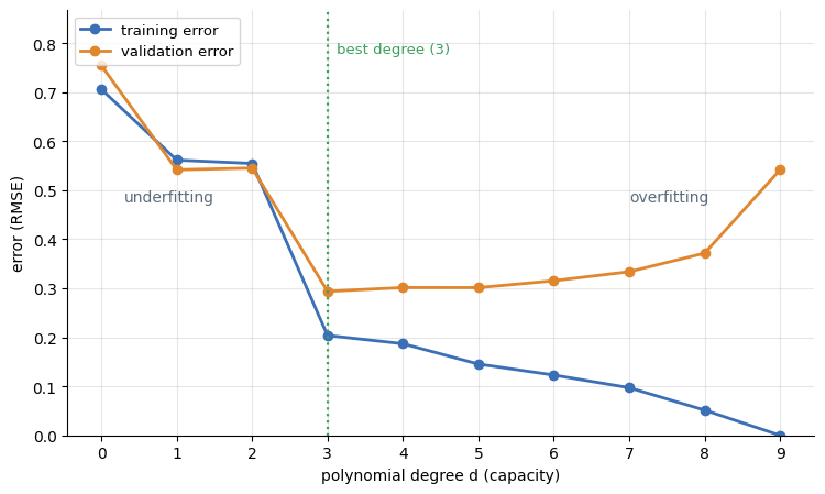
As the degree grows, the training error falls monotonically while the validation error falls, bottoms out, and rises again. The best degree sits at the bottom of the U.
This is the bias-variance trade-off. A rigid model is biased: it is systematically off, whichever sample it is trained on. A flexible model has high variance: its fit swings with every resample of the noise. Raising capacity trades bias for variance, and generalization is best where the two balance.
Remark: training error is not evidence of quality. Past the sweet spot it is evidence of memorization, and only performance on unseen data can tell the difference.
2.4 Regularization
Choosing the degree is a coarse dial: capacity jumps by whole integers. A finer control keeps a flexible family but makes complexity expensive inside the cost itself, by adding a penalty \(\Omega(w)\) scaled by a strength \(\lambda \ge 0\):
\[\boxed{\,J_\lambda(w)=\sum_{i=1}^{m} L\!\left(h_w(x^{(i)}),\,y^{(i)}\right) + \lambda\,\Omega(w)\,}\]The classic choice is the squared norm \(\Omega(w) = \lVert w \rVert_2^2\), the ridge penalty. The degree-9 fit only weaves through every point by using huge coefficients that cancel each other between the training points. The penalty makes those coefficients costly, so the minimizer trades a little training error for a much smoother curve. At \(\lambda = 0\) the overfitted fit returns, as \(\lambda \to \infty\) the curve flattens toward underfitting: \(\lambda\) sweeps the same bias-variance dial as the degree, but continuously.
Remark: regularization does not decide the right complexity for you, it converts a discrete choice (\(d\)) into a continuous one (\(\lambda\)) that is easier to tune. \(\lambda\) is a hyperparameter like the degree, chosen by the validation machinery of the next section. Where the penalty comes from (a prior on \(w\), via maximum a posteriori) and what the L1 variant adds are the subjects of Probabilistic formulation and Linear regression.
2.5 Hyperparameters, validation, and cross-validation
2.5.1 Training, validation, and test sets
Hyperparameters cannot be chosen on the training error, which only rewards more capacity. The fix is to keep data the model never touched during fitting. The standard split has three disjoint roles:
| Set | Used for | Touched |
|---|---|---|
| Training | fitting the model parameters | every fit |
| Validation | choosing the model and its hyperparameters | many times |
| Test | reporting one honest final estimate | exactly once |
Remark: the test set is sacred. Every time a choice is guided by test performance, the test set quietly becomes part of training and its estimate turns optimistic.
2.5.2 Cross-validation
Samples are often small, and a single train/validation split both wastes data and gives a noisy estimate. k-fold cross-validation reuses the data: partition it into \(K\) folds, and for each fold train on the other \(K-1\) and validate on the held-out fold. The cross-validation error averages the \(K\) rounds:
\[\boxed{ \text{CV}_K = \frac{1}{K}\sum_{k=1}^{K} \frac{1}{|F_k|}\sum_{i \in F_k} L\!\left(h^{(-k)}(x^{(i)}), y^{(i)}\right) }\]
where \(h^{(-k)}\) is trained on all folds except \(F_k\). Taking \(K = m\) gives leave-one-out cross-validation. Common choices are \(K = 5\) or \(K = 10\), trading computation against a lower-variance estimate.
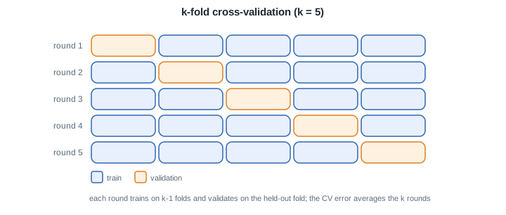
Each round holds out one fold for validation and trains on the rest, and the reported score is the average across folds.
2.5.3 Model and hyperparameter selection
Cross-validation is how we tune. Fit each candidate (a model family, a tree depth, the polynomial degree \(d\), or the penalty \(\lambda\)) and keep the one with the lowest validation or CV error. Only then, once the choice is frozen, do we touch the test set to report a final number.
Remark: choosing the winner on the test set inflates the estimate. With enough candidates one will look good by chance alone, the winner's curse, so selection and final evaluation must use different data.
2.6 Regression metrics: how far off, on average
The U-curve of section 2.3 already used a regression metric without naming it: the RMSE. For regression the raw material is the residual \(y - \hat{y}\) between the label and the prediction \(\hat{y} = h_w(x)\), and the metrics differ in how they aggregate the residuals, here for five predictions:
| \(y\) | \(\hat{y}\) | \(y - \hat{y}\) | |
|---|---|---|---|
| example 1 | 10 | 12 | \(-2\) |
| example 2 | 14 | 13 | \(1\) |
| example 3 | 8 | 9 | \(-1\) |
| example 4 | 12 | 9 | \(3\) |
| example 5 | 16 | 17 | \(-1\) |
| Metric | Formula | Here | Reads as |
|---|---|---|---|
| MSE | \(\frac{1}{m}\sum_i \left(y^{(i)} - \hat{y}^{(i)}\right)^2\) | \(3.2\) | the squared-error loss itself, in squared units |
| RMSE | \(\sqrt{\text{MSE}}\) | \(\approx 1.8\) | typical error, in the target's own units |
| MAE | \(\frac{1}{m}\sum_i \left\lvert y^{(i)} - \hat{y}^{(i)} \right\rvert\) | \(1.6\) | average miss, robust to outliers |
| \(R^2\) | \(1 - \sum_i \left(y^{(i)} - \hat{y}^{(i)}\right)^2 \big/ \sum_i \left(y^{(i)} - \bar{y}\right)^2\) | \(0.6\) | variance explained, against predicting the mean |
The mean here is \(\bar{y} = 12\). Squaring makes the MSE and RMSE quadratic in each residual, so one large error dominates them, while the MAE grows only linearly:
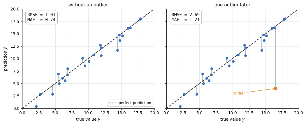
The same fit before and after a single outlier: the RMSE nearly triples while the MAE moves far less. Whether that sensitivity is a feature or a flaw depends on how costly large errors are in the application.
Remark: \(R^2\) compares the model against the laziest baseline, predicting the mean \(\bar{y}\) for every input. \(R^2 = 1\) is a perfect fit, \(R^2 = 0\) is no better than the baseline, and a negative \(R^2\), worse than the baseline, is validation's way of saying the model learned nothing. Unlike the RMSE and MAE it is scale-free, so it compares across targets in different units.
2.7 Classification metrics: beyond a single error rate
For classification, the number the validation reports need not be the raw loss. A trained classifier makes four kinds of calls: true and false positives, true and false negatives. Counting them on held-out data gives the confusion matrix, here for 29 examples:
| predicted \(+\) | predicted \(-\) | total | |
|---|---|---|---|
| actually \(+\) | TP = 11 | FN = 3 | 14 |
| actually \(-\) | FP = 5 | TN = 10 | 15 |
Every headline metric is a ratio of these four cells:
| Metric | Formula | Here | Reads as |
|---|---|---|---|
| Accuracy | \((TP+TN)/\text{total}\) | \(21/29 \approx 0.72\) | fraction correct overall |
| Recall (true positive rate) | \(TP/(TP+FN)\) | \(11/14 \approx 0.79\) | positives that were found |
| Precision | \(TP/(TP+FP)\) | \(11/16 \approx 0.69\) | flagged positives that are right |
| Specificity | \(TN/(TN+FP)\) | \(10/15 \approx 0.67\) | negatives that were kept |
| False positive rate | \(FP/(FP+TN)\) | \(5/15 \approx 0.33\) | negatives that were flagged |
| F1 score | \(2\,\text{Pr}\cdot\text{Re}/(\text{Pr}+\text{Re})\) | \(\approx 0.73\) | precision-recall balance |
Remark: accuracy alone can mislead. With 1% positives, always predicting "negative" scores 99% accuracy while finding nothing. Precision and recall keep score where it matters.
A classifier that outputs a score or a probability does not produce one confusion matrix but a family of them: sliding the decision threshold trades false positives against false negatives.
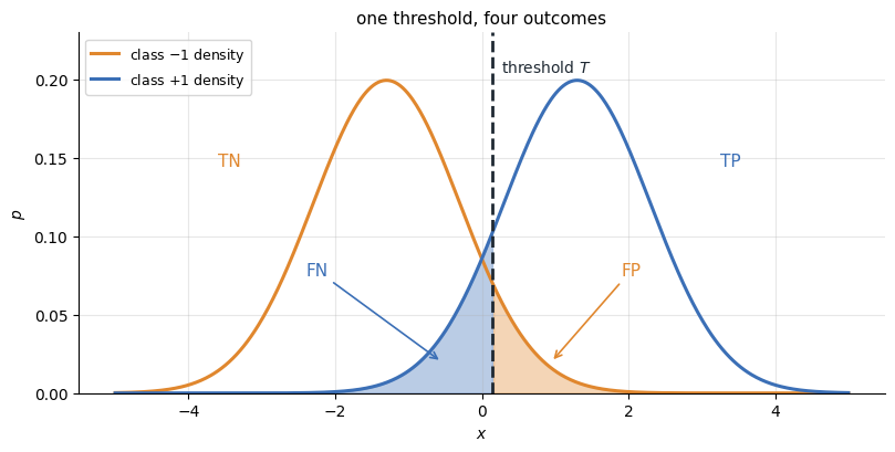
Everything right of the threshold is called positive. Pushing the threshold right shrinks the false positives (orange area) but grows the false negatives (blue area), and vice versa.
Sweeping the threshold and plotting the trade-off gives the ROC curve (recall against false positive rate, perfect is the top-left corner) and the precision-recall curve (perfect is the top-right corner). Two classifiers are compared by their whole curves, or by the area under them, rather than by a single threshold's numbers.
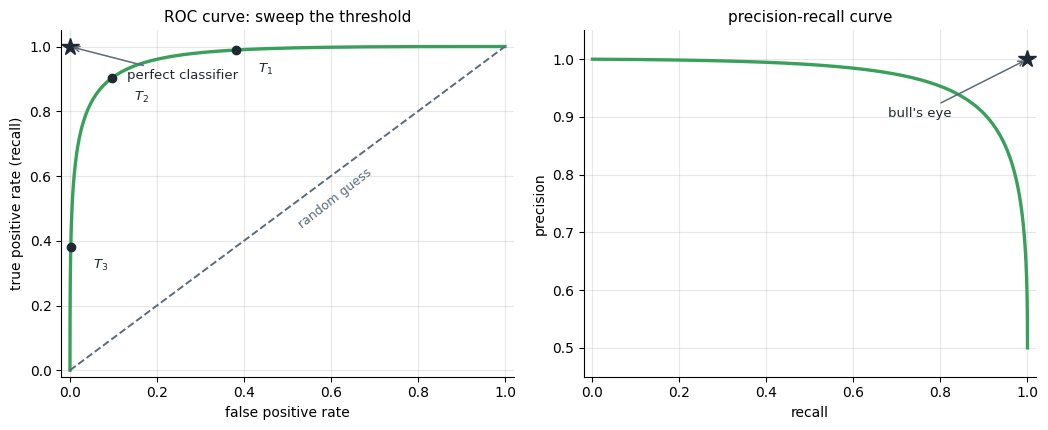
Each point on a curve is one threshold: \(T_1\) permissive, \(T_3\) strict. The closer the curve bends toward its perfect corner, the better the classifier at every trade-off.
Remark: this is what "a metric matched to the problem" means: compute these on the validation folds above to choose a model, and once, on the test set, to report it.
2.8 Common validation pitfalls
Honest validation is harder than it looks, and real data often breaks the usual assumptions in three ways.
- Data leakage. Information about the target leaks into the features. Standardizing with statistics computed on the full sample, or including a variable realized after the outcome, lets the model peek at the answer. Any preprocessing must be fit on the training folds only.
- Look-ahead bias. Using information that was not yet available at the moment of prediction, which arises whenever the data is time-ordered, produces backtests that cannot be reproduced live.
- Dependence. Many datasets are serially correlated (time series) or grouped (several observations that share a unit). Shuffling them into random folds mixes near-identical neighbours across train and validation, so the estimate is far too optimistic.
For time series, use a rolling-origin (blocked) scheme so the model is only ever tested on data that comes after its training window. For grouped data, hold out whole units (grouped cross-validation) so no unit appears on both sides.
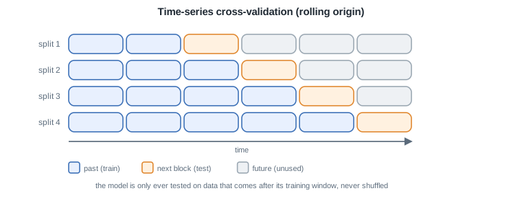
In a rolling-origin scheme the training window grows forward in time and the model is validated on the next block, never on shuffled data.
Remark: the honest question behind every split is the same. Would this have been knowable at the time, from data the model actually had?
2.9 The curse of dimensionality
Everything above rests on the sample standing in for the population near the points that matter. In high dimension that assumption degrades, and it degrades fast. Suppose the inputs fill the unit hypercube \([0,1]^d\) and we want a neighbourhood around a point that captures a fraction \(r\) of the data. A sub-cube containing a fraction \(r\) of the volume must have edge length:
\[\boxed{ e_d(r) = r^{1/d} }\]In one dimension, capturing 1% of the volume takes 1% of the axis. In \(d = 10\) dimensions it takes \(0.01^{1/10} \approx 0.63\), so 63% of the range of every feature, and in \(d = 100\) dimensions 95%. A neighbourhood that sees any reasonable share of the data stops being local, and methods that rely on nearby examples lose their footing. Filling space directly is hopeless too: covering each axis with just 10 bins already produces \(10^d\) cells, so the sample size needed to populate them grows exponentially with \(d\).
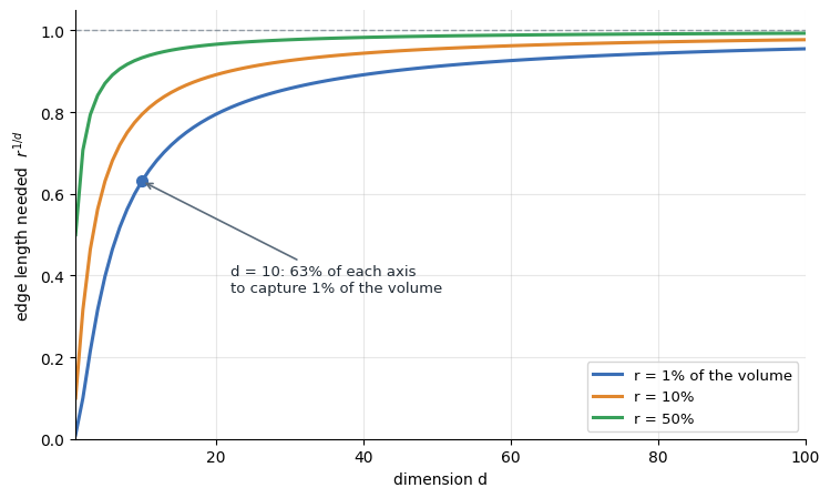
The edge length needed to capture a fixed fraction of the volume shoots toward 1 as the dimension grows: in high dimension, a "local" neighbourhood spans most of every axis.
Two more symptoms follow from the same geometry. Almost all of the volume of a high-dimensional cube sits near its boundary, so a typical point has no interior around it. And pairwise distances concentrate: the nearest and the farthest neighbour end up almost equally far, so distance itself becomes less informative.
Remark: this is why learning in high dimension leans on structure rather than raw proximity: linear models, regularization pulling toward simple fits, and features or embeddings that compress the inputs. Real data usually concentrates near a much lower-dimensional structure, and that is what makes learning possible at all.
The concepts are in place: fitting minimizes a loss, generalizing is the goal, validation measures it, and regularization with hyperparameter tuning controls it. The next module builds the probabilistic language (Bayes' rule, entropy, likelihood) behind the first concrete models.