
1. Introduction
Machine learning builds models that learn patterns from data instead of being explicitly programmed with rules. This module fixes the notation used throughout the course and maps the landscape of problems and models, so later modules can stay terse and formula-first.
1.1 Types of learning
- Supervised: learn from labelled examples (regression, classification).
- Unsupervised: find structure in unlabelled data (clustering, dimensionality reduction).
- Reinforcement: learn from feedback by interacting with an environment.
1.2 The workflow
- Define the problem and gather data.
- Explore and preprocess the data.
- Train candidate models.
- Evaluate and compare them.
- Deploy and monitor (see the MLOps course).
Objectives
- Fix the notation used across the whole course.
- Define the training set, the hypothesis, and the design matrix.
- Adopt the intercept convention \(x_0 = 1\).
- Classify a supervised problem by the type of its output.
- Distinguish discriminative from generative models.
1.3 Notation and setup
1.3.1 Training set
The training set is defined as a collection of \(m\) labelled examples:
\[\boxed{ \{(x^{(i)}, y^{(i)})\}_{i=1}^{m} }\]Symbols:
- \(x^{(i)}\) is the input (feature vector) of the \(i\)-th example.
- \(y^{(i)}\) is its target (label).
- \(m\) is the number of training examples.
- \(n\) is the number of features.
- \(x_j^{(i)}\) is the \(j\)-th feature of the \(i\)-th example.
Remark: the superscript \((i)\) indexes the example and the subscript \(j\) indexes the feature, so \(x_j^{(i)}\) is feature \(j\) of example \(i\).
By convention the input is augmented with a constant intercept term \(x_0 = 1\), so \(x \in \mathbb{R}^{n+1}\) and the parameters are \(\theta \in \mathbb{R}^{n+1}\).
\[\boxed{ x_0 = 1, \quad x \in \mathbb{R}^{n+1}, \quad \theta \in \mathbb{R}^{n+1} }\]Remark: the intercept lets a single dot product \(\theta^T x\) carry the bias term, so no separate constant has to be written.
1.3.2 Hypothesis
A hypothesis is defined as a function chosen from a model family that maps an input to a prediction:
\[\boxed{ h_\theta : x \mapsto h_\theta(x) }\]Learning is the search, over the parameters \(\theta\), for the hypothesis that best fits the training set.
1.3.3 Design matrix
The design matrix stacks the \(m\) transposed inputs row by row, and the target vector collects the labels:
\[\boxed{ X = \begin{bmatrix} (x^{(1)})^{T} \\ \vdots \\ (x^{(m)})^{T} \end{bmatrix}, \quad y = \begin{bmatrix} y^{(1)} \\ \vdots \\ y^{(m)} \end{bmatrix} }\]Here \(X \in \mathbb{R}^{m \times (n+1)}\) (each augmented input is a row) and \(y \in \mathbb{R}^{m}\).
Remark: with this layout many models reduce to compact matrix expressions, for example a linear prediction over all examples is \(X\theta\).
1.4 Types of problems and models
1.4.1 Type of prediction
A supervised problem is named by the nature of its target \(y\).
| Type | Target | Goal |
|---|---|---|
| Regression | \(y \in \mathbb{R}\) | predict a continuous value |
| Classification | \(y \in \{1, \dots, k\}\) | predict one of \(k\) discrete classes |
Remark: binary classification is the case \(k = 2\), often coded as \(y \in \{0, 1\}\) or \(y \in \{-1, +1\}\).
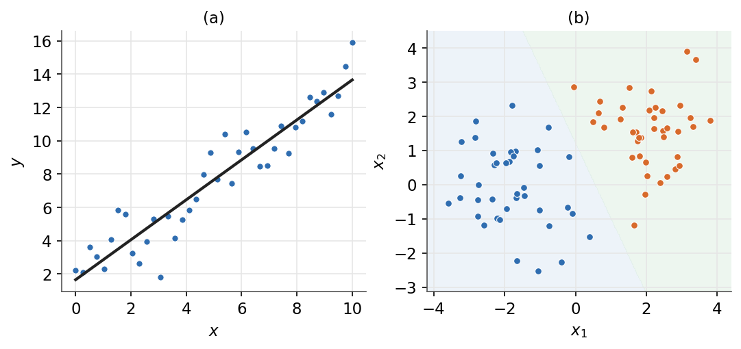
Left: regression fits a continuous output. Right: classification separates the input space into classes.
1.4.2 Type of model
A model is discriminative if it learns the conditional \(p(y \mid x)\) directly, and generative if it models how the data are generated, \(p(x \mid y)\) and \(p(y)\), then inverts via Bayes' rule:
\[\boxed{ p(y \mid x) = \frac{p(x \mid y)\, p(y)}{p(x)} }\]| Aspect | Discriminative | Generative |
|---|---|---|
| Goal | model the boundary between classes | model how each class generates data |
| What is learned | \(p(y \mid x)\) directly | \(p(x \mid y)\) and \(p(y)\), then Bayes |
| Examples | logistic regression, SVM | Gaussian discriminant analysis, naive Bayes |
Remark: \(p(x)\) is the same for every class, so for classification it can be dropped and the most probable class taken via \(\arg\max_y\, p(x \mid y)\, p(y)\).
1.4.3 Putting it together
The output type fixes regression vs classification, and the modelling choice fixes discriminative vs generative. Together they select a model family.
graph TD
  A["supervised problem"] --> B{"output type?"}
  B -->|"continuous"| C["regression"]
  B -->|"discrete"| D["classification"]
  D --> E{"model type?"}
  E -->|"discriminative"| F["logistic regression, SVM"]
  E -->|"generative"| G["GDA, naive Bayes"]
With the problem framed and the notation fixed, the next part introduces the tools used to fit a model to data: loss functions, gradient descent, and maximum likelihood.
Next: General concepts · Course overview