
# 1. Introduction Machine learning builds models that learn patterns from data instead of being explicitly programmed with rules. This module fixes the notation used throughout the course and maps the kinds of problems it tackles, so later modules can stay terse and formula-first. ## 1.1 Types of learning Machine learning problems are usually sorted into three paradigms. What separates them is not the algorithm but the feedback available during training: a label for every example, no labels at all, or a reward that arrives through interaction. 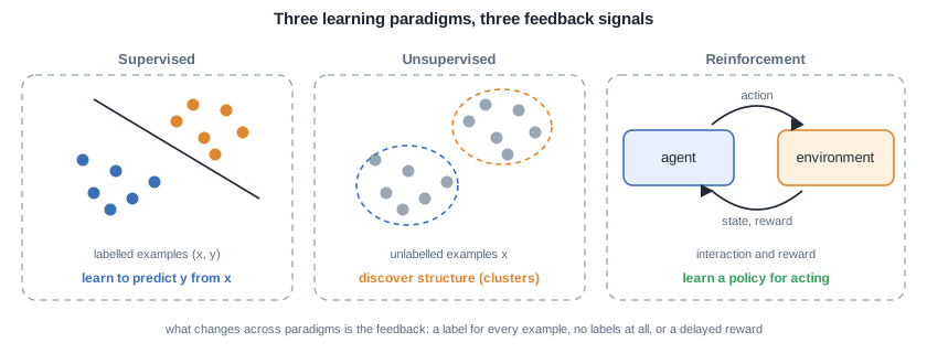 *Supervised learning fits a mapping from labelled examples, unsupervised learning finds structure in unlabelled data, and reinforcement learning improves a policy through interaction with an environment.* **Supervised learning.** Each training example pairs an input $x$ with the answer $y$ the model should produce, and the goal is a mapping $x \mapsto y$ that generalizes to inputs never seen in training. Predicting the price of a house from its features (regression) and deciding whether an email is spam (classification) are the canonical tasks. Labels make the objective explicit and progress measurable, which is why the theory is most developed here. Almost all of this course lives in this setting. **Unsupervised learning.** Only the inputs $x$ are available, and no label says what the right answer is. The goal shifts from prediction to description: group similar customers into segments (clustering), compress many correlated features into a few informative directions (dimensionality reduction), or estimate which regions of the input space are likely (density estimation). Success is harder to quantify, because there is no ground truth to compare against. **Reinforcement learning.** There is no fixed dataset at all. An agent takes an action, the environment returns a new state and a reward, and the reward may arrive long after the action that earned it. The goal is a policy, a rule for choosing actions that maximizes the cumulative reward. Game playing and robotics are the typical examples. It is a field of its own and sits outside the scope of this course. | Paradigm | Data | Feedback signal | What is learned | Canonical tasks | | --- | --- | --- | --- | --- | | Supervised | pairs $(x, y)$ | the label $y$ | a mapping $h : x \mapsto y$ | regression, classification | | Unsupervised | inputs $x$ only | none | structure in the data | clustering, dimensionality reduction | | Reinforcement | interaction | reward, often delayed | a policy for acting | control, game playing | *Remark:* the boundaries are not rigid. Semi-supervised learning mixes a few labelled examples with many unlabelled ones, and self-supervised learning manufactures labels from the data itself, for example by hiding a word and predicting it. Both reuse the supervised machinery introduced in this course. ## 1.2 The course notation ### 1.2.1 Training set The training set is defined as a collection of $m$ labelled examples: $$\boxed{ \{(x^{(i)}, y^{(i)})\}_{i=1}^{m} }$$ Symbols: - $x^{(i)}$ is the input (feature vector) of the $i$-th example. - $y^{(i)}$ is its target (label). - $m$ is the number of training examples. - $n$ is the number of features. - $x_j^{(i)}$ is the $j$-th feature of the $i$-th example. *Remark:* the superscript $(i)$ indexes the example and the subscript $j$ indexes the feature, so $x_j^{(i)}$ is feature $j$ of example $i$. By convention the input is augmented with a constant intercept term $x_0 = 1$, so $x \in \mathbb{R}^{n+1}$ and the parameters are $w \in \mathbb{R}^{n+1}$. $$\boxed{ x_0 = 1, \quad x \in \mathbb{R}^{n+1}, \quad w \in \mathbb{R}^{n+1} }$$ *Remark:* the intercept lets a single dot product $w^T x$ carry the bias term, so no separate constant has to be written. ### 1.2.2 Hypothesis A hypothesis is defined as a function chosen from a model family that maps an input to a prediction: $$\boxed{ h_w : x \mapsto \hat{y} = h_w(x) }$$ Two notations, two roles: $h_w$ names the function, and $\hat{y}$ names the value it predicts for one input, the hat marking an estimate of the label $y$. Learning is the search, over the parameters $w$, for the hypothesis that best fits the training set. ### 1.2.3 Design matrix The design matrix stacks the $m$ transposed inputs row by row, and the target vector collects the labels: $$\boxed{ X = \begin{bmatrix} (x^{(1)})^{T} \\ \vdots \\ (x^{(m)})^{T} \end{bmatrix}, \quad y = \begin{bmatrix} y^{(1)} \\ \vdots \\ y^{(m)} \end{bmatrix} }$$ Here $X \in \mathbb{R}^{m \times (n+1)}$ (each augmented input is a row) and $y \in \mathbb{R}^{m}$. *Remark:* with this layout many models reduce to compact matrix expressions, for example a linear prediction over all examples is $Xw$. ## 1.3 Types of problems A supervised problem is named by the nature of its target $y$. | Type | Target | Goal | | --- | --- | --- | | Regression | $y \in \mathbb{R}$ | predict a continuous value | | Classification | $y \in \{1, \dots, k\}$ | predict one of $k$ discrete classes | *Remark:* binary classification is the case $k = 2$, often coded as $y \in \{0, 1\}$ or $y \in \{-1, +1\}$. 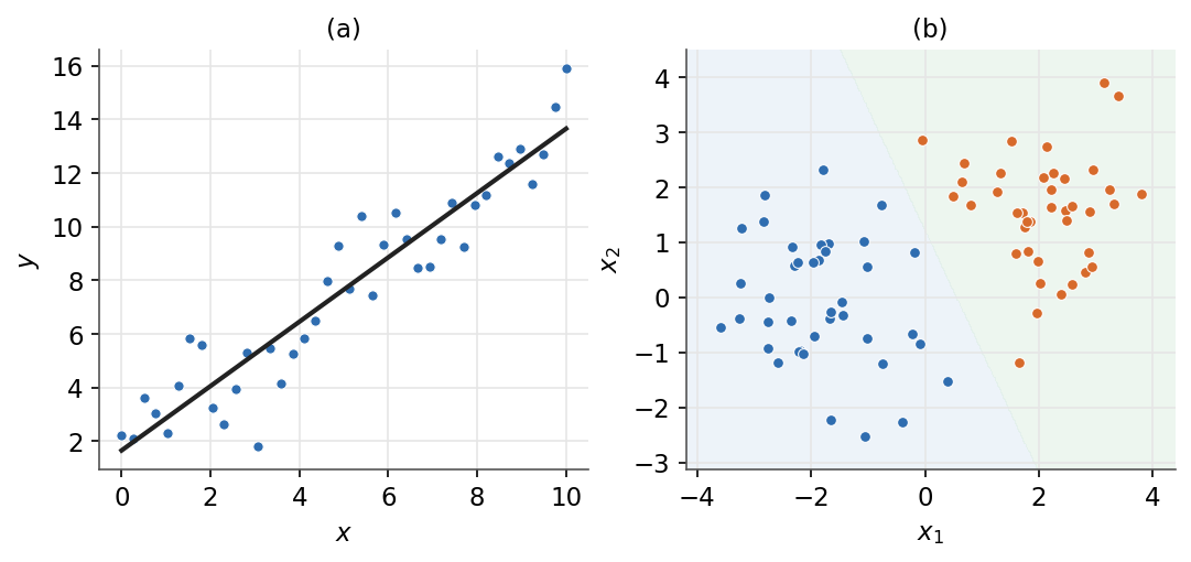 *Left: regression fits a continuous output. Right: classification separates the input space into classes.* *With the problem framed and the notation fixed, the next part turns to what learning really demands: minimizing a loss is easy, generalizing beyond the training set is the challenge.* --- Next: [General concepts](/en/Machine%20Learning/02%20General%20concepts) · [Course overview](/en/Machine%20Learning)