
Blame
|
1 | # 1. Introduction |
||||||
| 2 | ||||||||
|
3 | This course continues directly from the Machine Learning course, which closed the [Linear classification](/en/Machine%20Learning/05%20Linear%20classification) part with a key remark: a perceptron is a single unit, and stacked into layers it becomes a neural network. This lesson makes that bridge explicit. It recalls what one unit can do, shows the concrete task (XOR) where a single unit fails, and fixes the notation used throughout the rest of the course. |
||||||
|
4 | |||||||
| 5 | **Objectives** |
|||||||
| 6 | - Recall the perceptron as a single unit with a step activation and a linear boundary. |
|||||||
| 7 | - See why one unit cannot solve XOR, motivating hidden layers. |
|||||||
| 8 | - Understand what "deep" means and why hidden layers learn features. |
|||||||
| 9 | - Adopt the explicit-bias, per-layer notation used across this course. |
|||||||
| 10 | - Read a network as a composition of layer maps from input to prediction. |
|||||||
| 11 | ||||||||
| 12 | ## 1.1 The perceptron, recalled |
|||||||
| 13 | ||||||||
| 14 | The perceptron from the Machine Learning course is a single computational unit. It scores an input with a linear combination of its features and passes that score through a hard threshold. With parameters $\theta$ and the step activation $g$, its hypothesis is: |
|||||||
| 15 | ||||||||
| 16 | $$\boxed{ h(x) = g(\theta^T x), \quad g(z) = \begin{cases} 1 & \text{if } z \ge 0 \\ 0 & \text{otherwise} \end{cases} }$$ |
|||||||
| 17 | ||||||||
| 18 | The equation $\theta^T x = 0$ is a hyperplane, so the perceptron splits the input space with a single flat boundary. Points on one side are labelled $1$, points on the other are labelled $0$. |
|||||||
| 19 | ||||||||
| 20 | *Remark:* the boundary is linear because the score $\theta^T x$ is linear in $x$. The threshold only chooses a side, it does not bend the boundary. |
|||||||
| 21 | ||||||||
| 22 | ## 1.2 Why one unit is not enough |
|||||||
| 23 | ||||||||
| 24 | A single linear boundary can only solve problems whose classes are **linearly separable**, that is, separable by one straight cut. Many simple problems are, but not all. The classic counterexample is the exclusive-or (XOR) function of two binary inputs. |
|||||||
| 25 | ||||||||
| 26 | The truth tables below compare AND, OR, and XOR: |
|||||||
| 27 | ||||||||
| 28 | | $x_1$ | $x_2$ | AND | OR | XOR | |
|||||||
| 29 | | --- | --- | --- | --- | --- | |
|||||||
| 30 | | 0 | 0 | 0 | 0 | 0 | |
|||||||
| 31 | | 0 | 1 | 0 | 1 | 1 | |
|||||||
| 32 | | 1 | 0 | 0 | 1 | 1 | |
|||||||
| 33 | | 1 | 1 | 1 | 1 | 0 | |
|||||||
| 34 | ||||||||
| 35 | 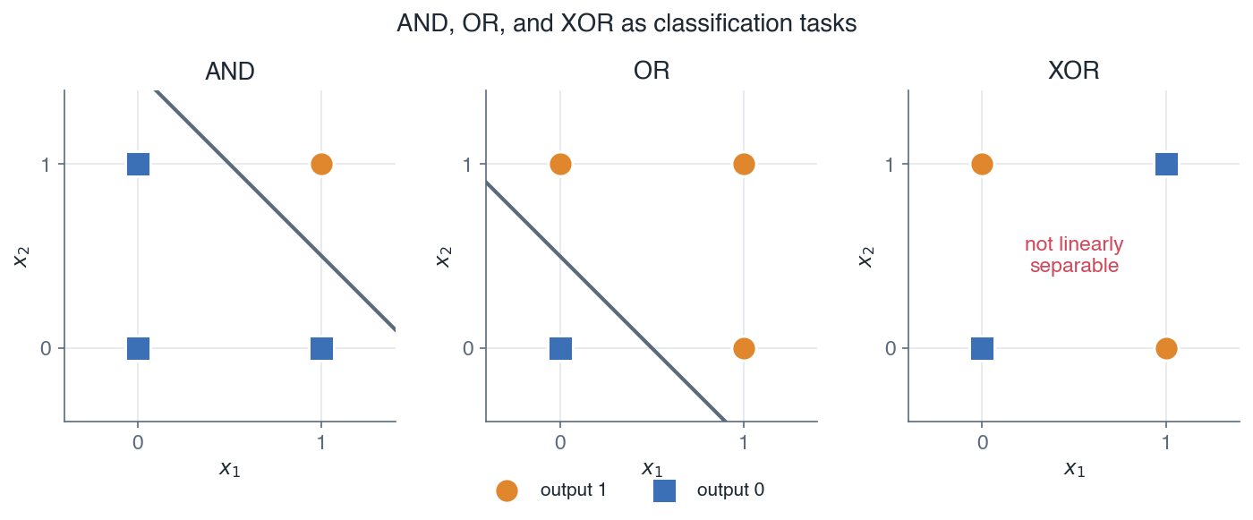 |
|||||||
| 36 | ||||||||
| 37 | *AND and OR are separable by a single straight line, but XOR is not, which is why one unit cannot solve it.* |
|||||||
| 38 | ||||||||
| 39 | For AND and OR the two output classes can be separated by a single line, so a perceptron solves them. For XOR the positive points $(0,1)$ and $(1,0)$ sit on one diagonal and the negative points $(0,0)$ and $(1,1)$ sit on the other. No single straight line can separate them. |
|||||||
| 40 | ||||||||
| 41 | *Remark:* XOR is not a special curiosity. It shows that some patterns are inherently nonlinear, so any model built from one linear boundary is fundamentally limited. The fix is to combine several units. |
|||||||
| 42 | ||||||||
| 43 | If we place a layer of units between the input and the output, the first units can carve the space with several boundaries and a later unit can combine their outputs. Two lines can isolate the XOR pattern where one cannot. That intermediate layer is a **hidden layer**, and it is what turns a single unit into a network. |
|||||||
| 44 | ||||||||
| 45 | ## 1.3 From units to networks |
|||||||
| 46 | ||||||||
| 47 | Stacking units into layers, and layers into a pipeline, gives a **neural network**. A network is **deep** when it has more than one hidden layer between the input and the output. Each layer applies a linear map followed by a nonlinear activation, and the layers are composed so the output of one feeds the input of the next. |
|||||||
| 48 | ||||||||
| 49 | The payoff is **representation learning**. In classical machine learning we hand-craft features, then feed them to a linear model. In a deep network the hidden layers learn their own features from raw input: early layers capture simple patterns and later layers combine them into more abstract ones. We specify the architecture and the objective, and the network discovers the intermediate representations by training. |
|||||||
| 50 | ||||||||
| 51 | *Remark:* stacking linear maps alone would collapse back to a single linear map, so the nonlinear activation $g$ between layers is essential. Without it, no depth would add expressive power. Activation functions are covered in the next lessons. |
|||||||
| 52 | ||||||||
| 53 | ## 1.4 Notation for this course |
|||||||
| 54 | ||||||||
| 55 | The Machine Learning course folded the bias into the score with the intercept convention $x_0 = 1$, so a single dot product $\theta^T x$ carried the constant term. This course keeps the bias **explicit** and uses a separate weight matrix per layer. This is the seam between the two courses: from here on, no augmented input and no folded bias. |
|||||||
| 56 | ||||||||
| 57 | ### 1.4.1 A single unit |
|||||||
| 58 | ||||||||
| 59 | With explicit bias, one unit has a weight vector $w$ and a scalar bias $b$. Its activation is: |
|||||||
| 60 | ||||||||
| 61 | $$\boxed{ a = g(w^T x + b) }$$ |
|||||||
| 62 | ||||||||
| 63 | The score $w^T x + b$ is the same affine function as before, only now the bias $b$ is written out instead of hidden inside $\theta$. |
|||||||
| 64 | ||||||||
| 65 | ### 1.4.2 A layer and a network |
|||||||
| 66 | ||||||||
| 67 | Group the units of layer $l$ into a weight matrix $W^{[l]}$ and a bias vector $b^{[l]}$. The layer computes a pre-activation $z^{[l]}$, then an activation $a^{[l]}$: |
|||||||
| 68 | ||||||||
| 69 | $$\boxed{ z^{[l]} = W^{[l]} a^{[l-1]} + b^{[l]}, \quad a^{[l]} = g^{[l]}(z^{[l]}) }$$ |
|||||||
| 70 | ||||||||
| 71 | The input feeds the first layer as $a^{[0]} = x$, and for an $L$-layer network the prediction is the last activation: |
|||||||
| 72 | ||||||||
| 73 | $$\boxed{ a^{[0]} = x, \quad \hat{y} = a^{[L]} }$$ |
|||||||
| 74 | ||||||||
| 75 | So the network is a composition of layer maps: $x = a^{[0]} \mapsto a^{[1]} \mapsto \cdots \mapsto a^{[L]} = \hat{y}$. |
|||||||
| 76 | ||||||||
| 77 | ### 1.4.3 Symbol table |
|||||||
| 78 | ||||||||
| 79 | | Symbol | Meaning | Shape | |
|||||||
| 80 | | --- | --- | --- | |
|||||||
| 81 | | $L$ | number of layers | scalar | |
|||||||
| 82 | | $n_l$ | number of units in layer $l$ | scalar | |
|||||||
| 83 | | $W^{[l]}$ | weight matrix of layer $l$ | $n_l \times n_{l-1}$ | |
|||||||
| 84 | | $b^{[l]}$ | bias vector of layer $l$ | $n_l$ | |
|||||||
| 85 | | $z^{[l]}$ | pre-activation of layer $l$ | $n_l$ | |
|||||||
| 86 | | $a^{[l]}$ | activation of layer $l$ | $n_l$ | |
|||||||
| 87 | | $g^{[l]}$ | activation function of layer $l$ | applied elementwise | |
|||||||
| 88 | | $\hat{y}$ | prediction, equal to $a^{[L]}$ | $n_L$ | |
|||||||
| 89 | ||||||||
| 90 | *Remark:* the activation $g^{[l]}$ acts componentwise, so an elementwise product later on is written with the Hadamard symbol $\odot$. The superscript in brackets, $[l]$, indexes the layer, not an exponent. |
|||||||
| 91 | ||||||||
| 92 | The following diagram shows the smallest useful network: an input layer, one hidden layer, and an output layer. |
|||||||
| 93 | ||||||||
| 94 | 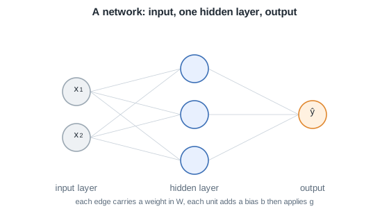 |
|||||||
| 95 | ||||||||
| 96 | *A neural network: an input layer, one hidden layer, and an output. Each edge carries a weight and each unit adds a bias then applies an activation g.* |
|||||||
| 97 | ||||||||
| 98 | Each arrow carries a weight from $W^{[l]}$, and every hidden and output unit adds its bias from $b^{[l]}$ before applying its activation. This two-unit hidden layer is exactly what lets the network solve XOR, the task that defeated a single unit. |
|||||||
| 99 | ||||||||
| 100 | *The next lesson formalizes this picture as the multilayer perceptron, writing the full forward pass layer by layer and choosing the activation functions.* |
|||||||
| 101 | ||||||||
| 102 | --- |
|||||||
| 103 | Next: [Multilayer perceptron](/en/Deep%20Learning/02%20Multilayer%20perceptron) · [Course overview](/en/Deep%20Learning) |
|||||||