Commit 81a3ca
2026-07-28 13:29:31 lugonthier: slide 01| en/Machine Learning.md .. | |
| @@ 12,8 12,7 @@ | |
| 4. [Linear regression](/en/Machine%20Learning/04%20Linear%20regression) | |
| 5. [Linear classification](/en/Machine%20Learning/05%20Linear%20classification) | |
| 6. [Multilayer neural networks](/en/Machine%20Learning/06%20Multilayer%20neural%20networks) | |
| - | 7. [Support Vector Machines](/en/Machine%20Learning/07%20Support%20Vector%20Machines) |
| - | 8. [Decision trees and ensemble methods](/en/Machine%20Learning/08%20Decision%20trees%20and%20ensemble%20methods) |
| + | 7. [Decision trees and ensemble methods](/en/Machine%20Learning/07%20Decision%20trees%20and%20ensemble%20methods) |
| --- | |
| [MLOps](/en/MLOps) · [Home](/en) | |
| en/Machine Learning/02 General concepts.md .. | |
| @@ 18,7 18,6 @@ | |
| | --- | --- | --- | | |
| | Least squared error | $\tfrac{1}{2}(y-z)^2$ | Linear regression | | |
| | Logistic | $\log\!\left(1+\exp(-yz)\right)$ | Logistic regression | | |
| - | | Hinge | $\max(0,\,1-yz)$ | SVM | |
| | Cross-entropy | $-\left[\,y\log\hat{y}+(1-y)\log(1-\hat{y})\,\right]$ | Neural networks | | |
| *Remark:* $z$ denotes a raw score such as $w^T x$, whereas $\hat{y} \in (0,1)$ denotes a predicted probability, the model's estimate of the label $y$. The cross-entropy row takes a probability $\hat{y}$, not a raw score. | |
| en/Machine Learning/05 Linear classification.md .. | |
| @@ 70,7 70,7 @@ | |
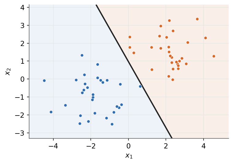
| 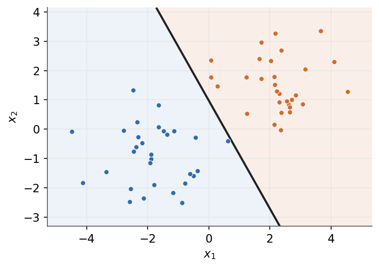 | |
| - | *The perceptron finds one separating hyperplane, not necessarily the maximum-margin one the support vector machine will choose.* |
| + | *The perceptron finds one separating hyperplane, not necessarily the one with the widest margin.* |
| ### 5.3.4 Multiclass perceptron | |
| @@ 94,7 94,7 @@ | |
| If the data is linearly separable the perceptron converges in a finite number of updates, otherwise the weights oscillate forever. And since the criterion is zero on every separating hyperplane, all of them count as "optimal", including those that graze the data. | |
| - | *Remark:* three upgrades fix these limits, and each one opens a module. A smooth activation and loss give logistic regression, next section. Margins and basis functions lead to the [Support Vector Machine](/en/Machine%20Learning/07%20Support%20Vector%20Machines). Stacking neurons into layers gives [multilayer neural networks](/en/Machine%20Learning/06%20Multilayer%20neural%20networks), the starting point of the Deep Learning course. |
| + | *Remark:* two upgrades fix these limits, and each one opens a module. A smooth activation and loss give logistic regression, next section. Stacking neurons into layers gives [multilayer neural networks](/en/Machine%20Learning/06%20Multilayer%20neural%20networks), the starting point of the Deep Learning course. |
| ## 5.4 Logistic regression | |
| @@ 246,7 246,7 @@ | |
| | Update | $w_j \leftarrow w_j - \alpha \sum_{i=1}^{m}\left(\hat{y}^{(i)} - y^{(i)}\right)x_j^{(i)}$ | | |
| | Multiclass | softmax $\hat{y}_c = \tfrac{\exp(w_c^T x)}{\sum_{j}\exp(w_j^T x)}$ and the categorical cross-entropy | | |
| - | *Remark:* read side by side, the perceptron update (in its $\{0, 1\}$ coding) and the logistic update are the same formula, the residual times the input, and only the activation changes (the step for the perceptron, the sigmoid for logistic regression, and the identity of linear regression completes the family). The Deep Learning course picks up exactly this thread, stacking such units into layers. One loss is deliberately missing from this menu, the hinge $\max(0,\,1 - y\,w^T x)$, which penalizes small margins as well as mistakes: it belongs to the [SVM](/en/Machine%20Learning/07%20Support%20Vector%20Machines). |
| + | *Remark:* read side by side, the perceptron update (in its $\{0, 1\}$ coding) and the logistic update are the same formula, the residual times the input, and only the activation changes (the step for the perceptron, the sigmoid for logistic regression, and the identity of linear regression completes the family). The Deep Learning course picks up exactly this thread, stacking such units into layers. |
| *With linear models covered, the next module stacks these building blocks into multilayer neural networks.* | |
| en/Machine Learning/06 Multilayer neural networks.md .. | |
| @@ 181,7 181,7 @@ | |
| </details> | |
| - | *This module is the doorway to the [Deep Learning](/en/Deep%20Learning) course, which picks the story up exactly here: the activation functions, the optimizers, initialization, normalization, regularization, and the architectures built on them. The next module returns to linear models from a new angle, the maximum-margin classifier.* |
| + | *This module is the doorway to the [Deep Learning](/en/Deep%20Learning) course, which picks the story up exactly here: the activation functions, the optimizers, initialization, normalization, regularization, and the architectures built on them. The next module changes tools entirely: decision trees, and the ensembles built from them.* |
| --- | |
| - | Next: [Support Vector Machines](/en/Machine%20Learning/07%20Support%20Vector%20Machines) · [Course overview](/en/Machine%20Learning) |
| + | Next: [Decision trees and ensemble methods](/en/Machine%20Learning/07%20Decision%20trees%20and%20ensemble%20methods) · [Course overview](/en/Machine%20Learning) |
| en/Machine Learning/08 Decision trees and ensemble methods.md .. en/Machine Learning/07 Decision trees and ensemble methods.md | |
| @@ 1,8 1,8 @@ | |
| - | # 8. Decision trees and ensemble methods |
| + | # 7. Decision trees and ensemble methods |
| Why trust one model when a committee can vote? This module builds the ensemble toolbox: the bootstrap and bagging to cut variance, AdaBoost to turn weak learners into a strong one, decision trees as the base learner of choice, and random forests as the combination that wins in practice. | |
| - | ## 8.1 Why a single model? |
| + | ## 7.1 Why a single model? |
| Every module so far trains one model and keeps it. A committee of $M$ models is almost always better than any single member. The combination is an average for regression and a majority vote for classification: | |
| @@ 15,11 15,11 @@ | |
| | Bagging | high capacity (deep trees) | in parallel, on resampled data | variance | | |
| | Boosting | low capacity (stumps) | sequentially, on reweighted data | bias | | |
| - | ## 8.2 The bootstrap: averaging away variance |
| + | ## 7.2 The bootstrap: averaging away variance |
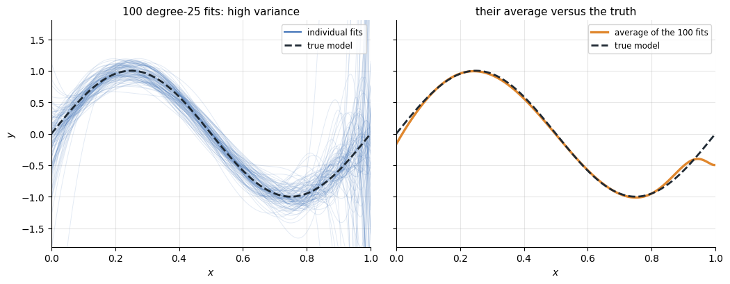
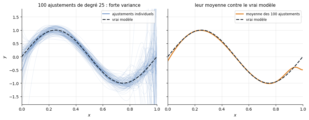
| Why does combining help? Train the same flexible model, a degree-25 polynomial, on 100 different training sets and the individual fits disagree wildly. Their average, however, hugs the true curve. | |
| - |  |
| + | 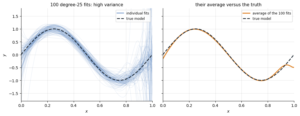 |
| *Left: 100 degree-25 fits, one per training set, each chasing its own noise. Right: their average is far closer to the truth, the fluctuations cancel.* | |
| @@ 33,11 33,11 @@ | |
| The same example can appear several times in one resample, and the probability that a given example never appears is $(1-\tfrac1N)^N\to e^{-1}\approx0.37$: about 37% of the data is left out of each resample. These are its out-of-bag (OOB) examples, which random forests will put to work below. | |
| - | ## 8.3 Bagging |
| + | ## 7.3 Bagging |
| Bagging (Bootstrap AGGregating) is the committee built from the bootstrap: resample $m$ training sets, train one model on each, combine the votes. | |
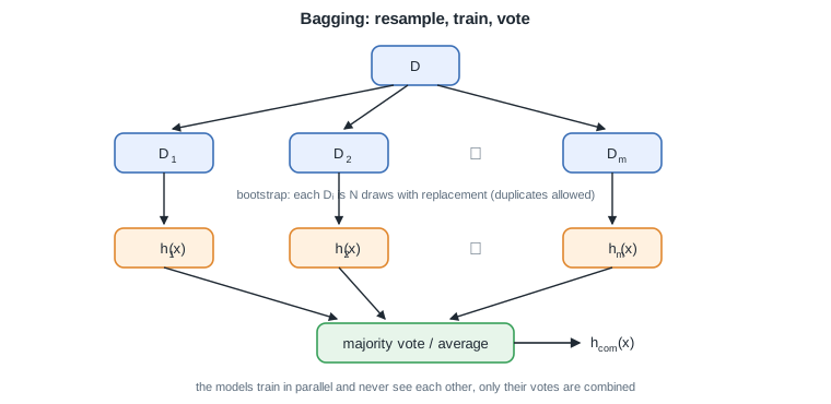
| - |  |
| + | 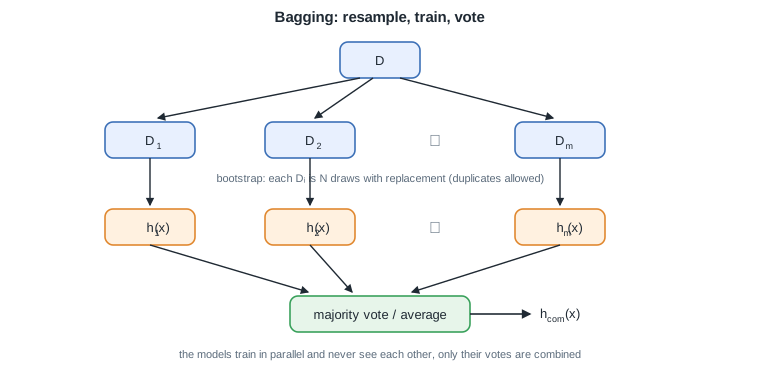 |
| *One dataset becomes $m$ bootstrap resamples, each trains its own model, and only the votes meet.* | |
| @@ 45,7 45,7 @@ | |
| *Remark:* averaging leaves bias unchanged while shrinking variance, so bagging suits base models with low bias and high variance, exactly the deep decision trees of section 8.5. A model that underfits stays underfitting after bagging. | |
| - | ## 8.4 Boosting: AdaBoost |
| + | ## 7.4 Boosting: AdaBoost |
| Boosting takes the opposite bet: combine many weak learners, models barely better than chance, into a strong one. The ensemble is a weighted sum built one learner at a time: | |
| @@ 57,7 57,7 @@ | |
| 2. There is **no bootstrap**: every example is used to train every learner. | |
| 3. The data is **reweighted**: examples misclassified by $h_t$ gain weight, so $h_{t+1}$ concentrates on them. | |
| - | ### 8.4.1 The algorithm |
| + | ### 7.4.1 The algorithm |
| With labels $y\in\{-1,+1\}$, keep one weight $w^{(i)}$ per example, initialized to $1/N$. At each round $t = 1, \dots, T$: | |
| @@ 73,13 73,13 @@ | |
| The final classifier is the weighted vote $H_T(x) = \mathrm{sign}\big(\sum_t \alpha_t h_t(x)\big)$. | |
| - |  |
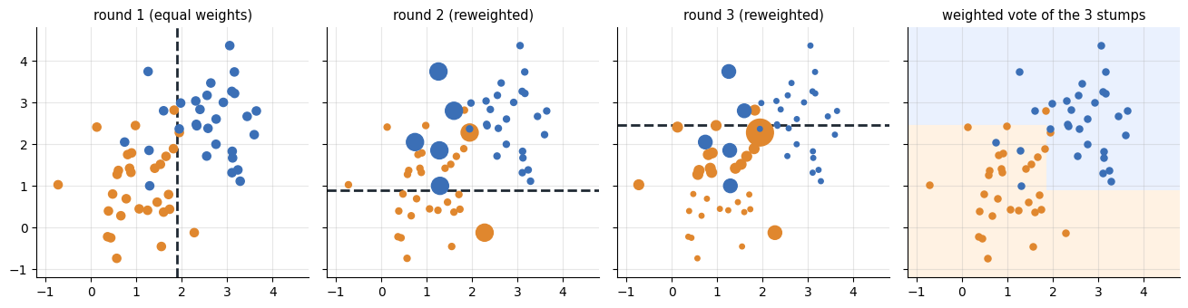
| + | 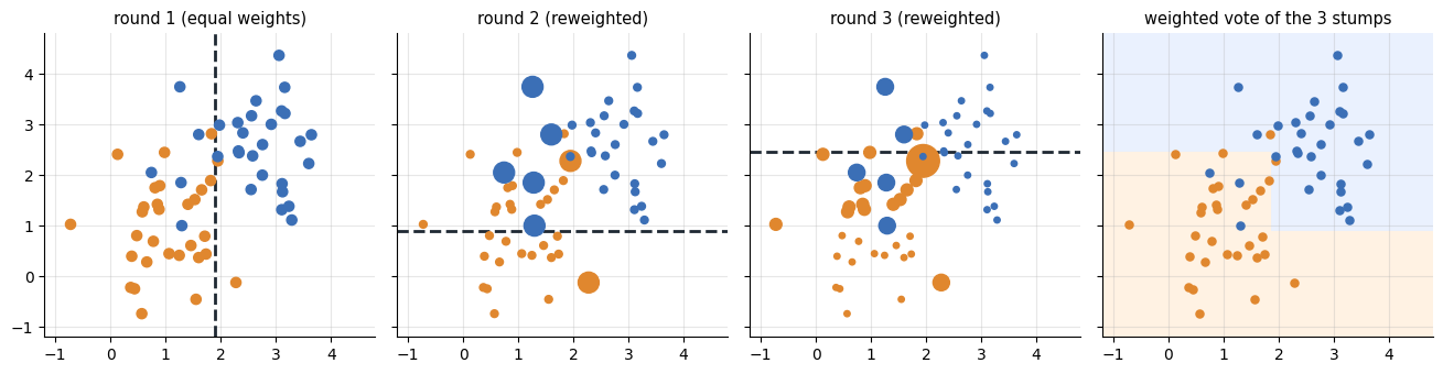 |
| *Each round fits one stump to the weighted data (dot size = weight). Misclassified points inflate, steering the next stump, and the weighted vote of three axis-aligned cuts already draws a jagged, nonlinear boundary.* | |
| *Remark:* the classic weak learner is the stump, a one-split tree perpendicular to an axis. Stumps are extremely fast, their combination gives the staircase boundaries above, and the learned $\alpha_t$ double as a ranking of useful features: the features whose stumps earn large votes are the informative ones. | |
| - | ### 8.4.2 Gradient boosting |
| + | ### 7.4.2 Gradient boosting |
| Gradient boosting generalizes the idea to any differentiable loss $L$. At stage $t$ it fits the next learner to the negative gradient of the loss evaluated at the current model, the pseudo-residual defined as | |
| @@ 98,17 98,17 @@ | |
| | mainly reduces | variance | bias | | |
| | reweighting | none (bootstrap) | weights or pseudo-residuals | | |
| - | ## 8.5 Decision trees |
| + | ## 7.5 Decision trees |
| - | ### 8.5.1 From stumps to trees |
| + | ### 7.5.1 From stumps to trees |
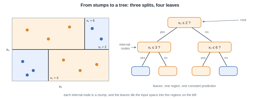
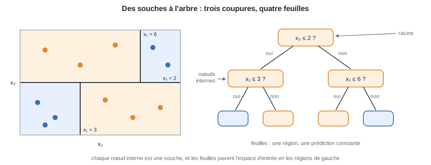
| A stump asks one question about one feature. Chain the questions, each answer leading to the next stump, and you get a decision tree: a root, internal nodes, and leaves that tile the input space. | |
| - |  |
| + | 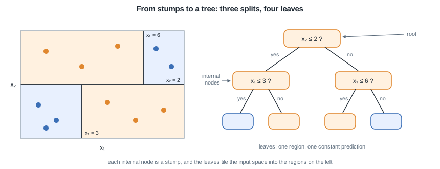 |
| *Three splits carve the plane into four regions (left), and the same three splits read as a tree (right): the root and internal nodes test features, the leaves predict.* | |
| - | ### 8.5.2 Tree as a partition |
| + | ### 7.5.2 Tree as a partition |
| A CART tree partitions the input space into $M$ disjoint regions $R_1,\dots,R_M$ (the leaves) and predicts a constant $c_m$ on each. The prediction is defined as | |
| @@ 118,11 118,11 @@ | |
| *Remark:* the regions are axis-aligned boxes, so the decision boundary is a staircase. A single tree has low bias but high variance: left unchecked it keeps splitting until it isolates every outlier. | |
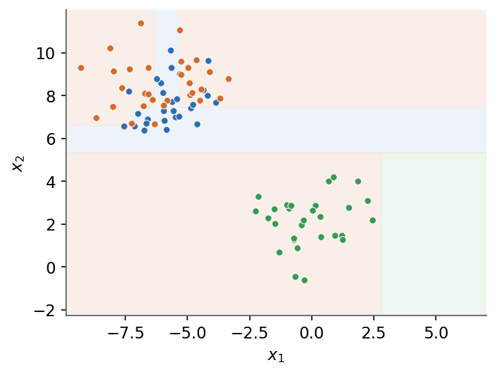
| - |  |
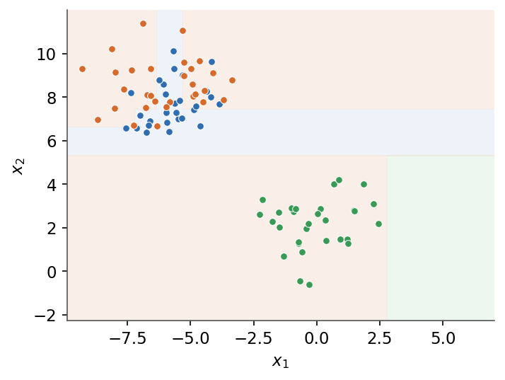
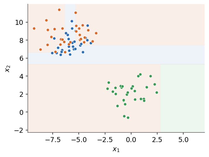
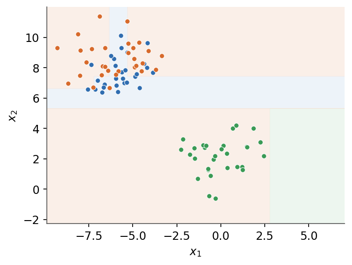
| + | 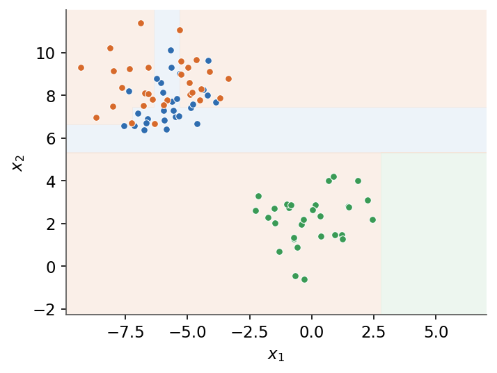 |
| *A tree carves the input space into axis-aligned regions, each with a constant prediction.* | |
| - | ### 8.5.3 Impurity and split selection |
| + | ### 7.5.3 Impurity and split selection |
| Which question should a node ask? The one that leaves the children as pure as possible. For a region with class proportions $\hat p_k$, impurity measures how mixed the labels are. The Gini index is defined as | |
| @@ 145,7 145,7 @@ | |
| *Remark:* the two criteria almost always pick the same split. Gini is the default in most implementations because it avoids the logarithm. | |
| - | ### 8.5.4 Regression trees |
| + | ### 7.5.4 Regression trees |
| For regression the leaf value is the mean of the targets in the region, defined as | |
| @@ 153,7 153,7 @@ | |
| and splits minimize the within-region squared error instead of a classification impurity. | |
| - | ### 8.5.5 Pruning |
| + | ### 7.5.5 Pruning |
| An unpruned tree fits the training set exactly and overfits. Cost-complexity pruning trades fit against tree size $|T|$ (the number of leaves) through a penalty $\alpha\ge0$: | |
| @@ 161,7 161,7 @@ | |
| Increasing $\alpha$ collapses the weakest splits, yielding a nested sequence of subtrees. The best $\alpha$ is chosen by the cross-validation of [General concepts](/en/Machine%20Learning/02%20General%20concepts). | |
| - | ## 8.6 Random forests |
| + | ## 7.6 Random forests |
| A random forest is bagging applied to deep trees, plus a second source of randomness. The variance formula of section 8.2 said the residual term $\rho\sigma^2$ survives averaging, so the trees must be decorrelated: at each split only a random subset of $m_{\text{try}}$ features is considered as split candidates. The usual choices are | |
| @@ 178,7 178,7 @@ | |
| | tree correlation $\rho$ | higher | lower | | |
| | variance reduction | moderate | stronger | | |
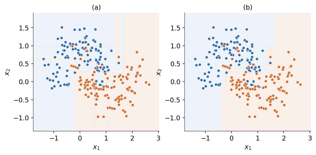
| - |  |
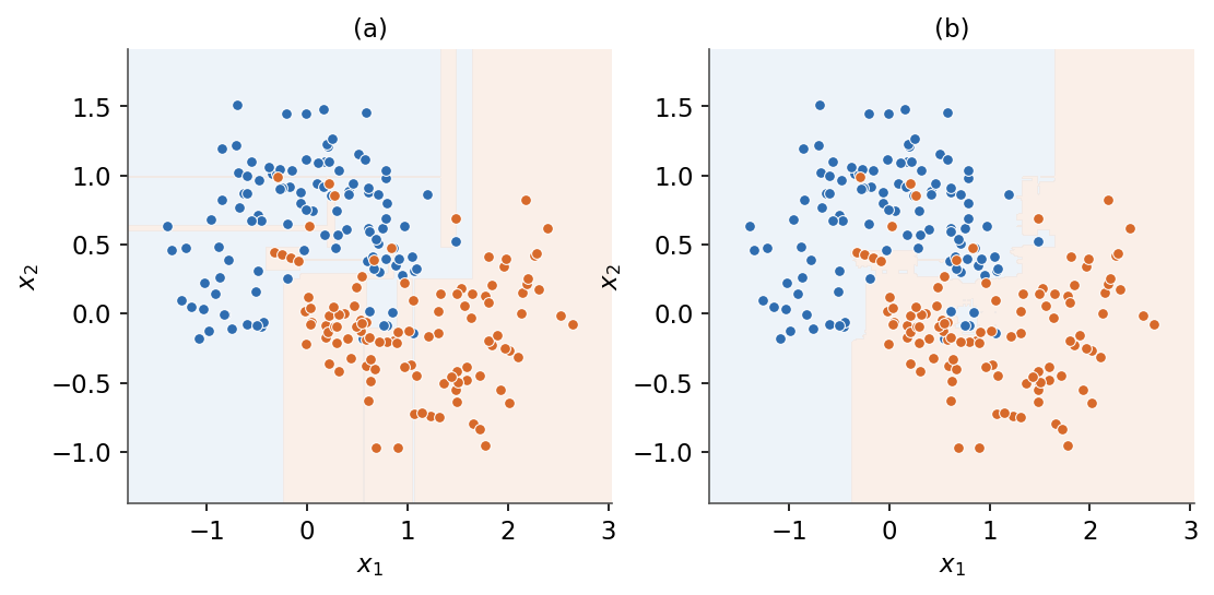
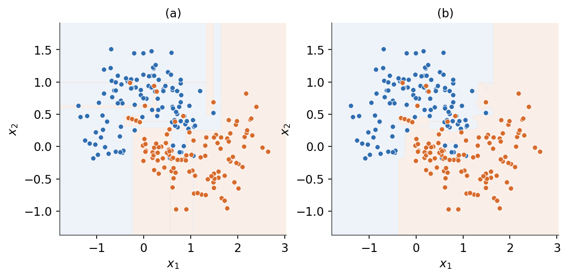
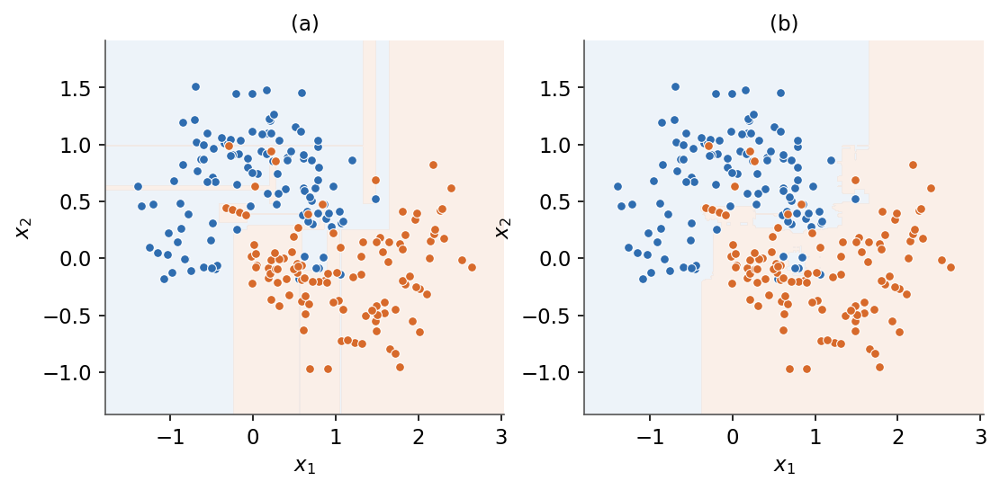
| + | 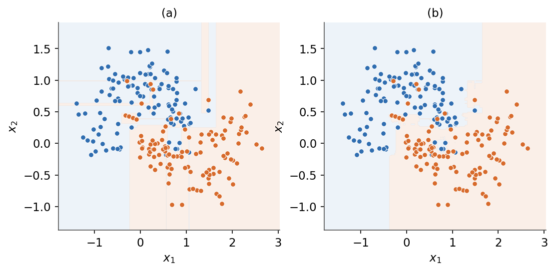 |
| *(a) A single deep tree overfits with a jagged boundary. (b) A random forest averages many trees for a smoother boundary.* | |
| en/Machine Learning/08 Decision trees and ensemble methods/adaboost-rounds.png .. en/Machine Learning/07 Decision trees and ensemble methods/adaboost-rounds.png | |
| en/Machine Learning/08 Decision trees and ensemble methods/bagging-pipeline.svg .. en/Machine Learning/07 Decision trees and ensemble methods/bagging-pipeline.svg | |
| en/Machine Learning/08 Decision trees and ensemble methods/forest-vs-tree.png .. en/Machine Learning/07 Decision trees and ensemble methods/forest-vs-tree.png | |
| en/Machine Learning/08 Decision trees and ensemble methods/tree-boundary.png .. en/Machine Learning/07 Decision trees and ensemble methods/tree-boundary.png | |
| en/Machine Learning/08 Decision trees and ensemble methods/tree-from-stumps.svg .. en/Machine Learning/07 Decision trees and ensemble methods/tree-from-stumps.svg | |
| en/Machine Learning/08 Decision trees and ensemble methods/variance-reduction.png .. en/Machine Learning/07 Decision trees and ensemble methods/variance-reduction.png | |
| en/Machine Learning/07 Support Vector Machines.md .. /dev/null | |
| @@ 1,209 0,0 @@ | |
| - | # 7. Support Vector Machines |
| - | |
| - | Support vector machines are large-margin linear classifiers. They pick the boundary that |
| - | maximizes the distance to the nearest points, control overfitting with the hinge loss and a |
| - | penalty $C$, and use kernels to fit nonlinear boundaries without ever forming the feature map. |
| - | Throughout, labels are $y \in \{-1,+1\}$ and the decision uses a raw score $z = w^T x - b$. |
| - | |
| - | ## 7.1 Optimal margin classifier |
| - | |
| - | Labels are $y \in \{-1,+1\}$, with weight vector $w \in \mathbb{R}^{n}$ and bias $b$. |
| - | |
| - | ### 7.1.1 Hypothesis and boundary |
| - | |
| - | The hypothesis is defined as the sign of the raw score $z = w^T x - b$: |
| - | |
| - | $$\boxed{ h(x) = \operatorname{sign}(w^T x - b) }$$ |
| - | |
| - | The decision boundary is the set of points with zero score: |
| - | |
| - | $$\boxed{ w^T x - b = 0 }$$ |
| - | |
| - | *Remark:* $w$ is orthogonal to the boundary, so it sets the orientation, and $b$ sets the offset. |
| - | |
| - | ### 7.1.2 Geometric margin |
| - | |
| - | The geometric margin of example $i$ is defined as its signed distance to the boundary, made |
| - | positive by the label: |
| - | |
| - | $$\boxed{ \gamma^{(i)} = y^{(i)} \, \frac{w^T x^{(i)} - b}{\lVert w \rVert} }$$ |
| - | |
| - | A correctly classified point has $\gamma^{(i)} > 0$. The margin of the dataset is the smallest |
| - | $\gamma^{(i)}$ over all examples. |
| - | |
| - | *Remark:* dividing by $\lVert w \rVert$ makes the margin invariant to rescaling $(w,b)$, unlike |
| - | the raw score $z$. |
| - | |
| - | ### 7.1.3 Hard-margin primal |
| - | |
| - | Fixing the scale so the closest points satisfy $y^{(i)}(w^T x^{(i)} - b) = 1$, maximizing the |
| - | margin is equivalent to minimizing $\lVert w \rVert^2$ subject to a unit functional margin: |
| - | |
| - | $$\boxed{ \min_{w,b} \tfrac{1}{2}\lVert w \rVert^2 \quad \text{s.t.} \quad y^{(i)}(w^T x^{(i)} - b) \ge 1 \ \ \forall i }$$ |
| - | |
| - | This is a convex quadratic program with linear constraints, so it has a unique optimum. |
| - | |
| - | *Remark:* it requires the data to be linearly separable. The next lesson relaxes that with slack |
| - | variables. |
| - | |
| - |  |
| - | |
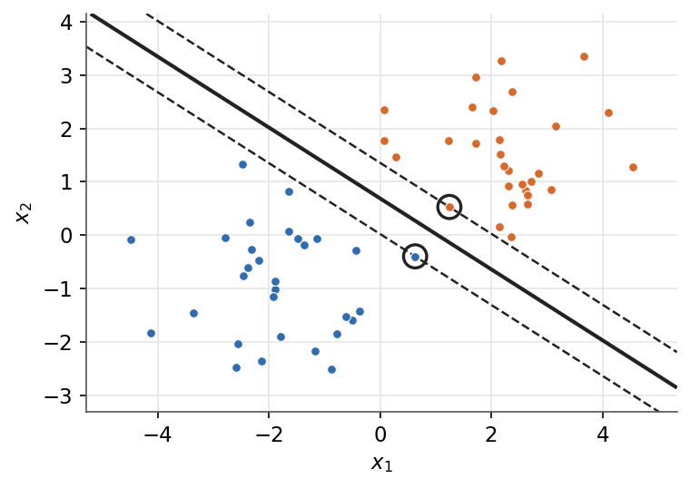
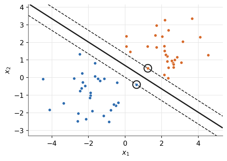
| - | *The optimal hyperplane (solid) maximizes the margin (dashed). Circled points are the support vectors.* |
| - | |
| - | ## 7.2 Hinge loss |
| - | |
| - | The raw score is $z = w^T x - b$ and labels are $y \in \{-1,+1\}$. |
| - | |
| - | ### 7.2.1 Hinge loss |
| - | |
| - | The hinge loss is defined as the amount by which the margin $yz$ falls short of $1$, clipped at zero: |
| - | |
| - | $$\boxed{ L(z,y) = \max(0,\, 1 - yz), \quad z = w^T x - b }$$ |
| - | |
| - | It is zero once $yz \ge 1$ (the point is correct and beyond the margin) and grows linearly inside |
| - | or past the margin. |
| - | |
| - | *Remark:* the hinge loss is convex but not differentiable at $yz = 1$, so it is optimized with |
| - | subgradients. |
| - | |
| - | ### 7.2.2 Soft-margin primal |
| - | |
| - | Introduce a slack $\xi_i \ge 0$ per example to allow margin violations, penalized by $C > 0$: |
| - | |
| - | $$\boxed{ \min_{w,b,\xi} \tfrac{1}{2}\lVert w \rVert^2 + C\sum_{i=1}^{m}\xi_i \quad \text{s.t.} \quad y^{(i)}(w^T x^{(i)} - b) \ge 1 - \xi_i, \ \ \xi_i \ge 0 }$$ |
| - | |
| - | At the optimum $\xi_i = \max(0,\, 1 - y^{(i)}(w^T x^{(i)} - b))$, so eliminating the slacks gives |
| - | the unconstrained regularized form: |
| - | |
| - | $$\boxed{ \min_{w,b} \tfrac{1}{2}\lVert w \rVert^2 + C\sum_{i=1}^{m}\max\!\big(0,\, 1 - y^{(i)}(w^T x^{(i)} - b)\big) }$$ |
| - | |
| - | This is regularization plus hinge loss: the $\tfrac{1}{2}\lVert w \rVert^2$ term widens the margin |
| - | and the sum penalizes violations. |
| - | |
| - | ### 7.2.3 Role of $C$ |
| - | |
| - | | $C$ | Penalty on violations | Margin | Behaviour | |
| - | | --- | --- | --- | --- | |
| - | | small | weak | wide | more violations tolerated, lower variance | |
| - | | large | strong | narrow | fewer violations, fits training data harder | |
| - | |
| - | *Remark:* as $C \to \infty$ no violation is tolerated, which recovers the hard-margin classifier. |
| - | |
| - | ## 7.3 Kernels |
| - | |
| - | ### 7.3.1 Kernel definition |
| - | |
| - | A kernel is defined as the inner product of a feature map $\phi$ applied to two inputs: |
| - | |
| - | $$\boxed{ K(x,z) = \phi(x)^T \phi(z) }$$ |
| - | |
| - | A valid kernel computes this inner product directly, so $\phi$ never has to be formed (it may even |
| - | be infinite-dimensional). |
| - | |
| - | ### 7.3.2 Kernel trick |
| - | |
| - | The SVM dual depends on the data only through inner products $\langle x^{(i)}, x^{(j)} \rangle$. |
| - | The kernel trick replaces each inner product with a kernel: |
| - | |
| - | $$\boxed{ \langle x^{(i)}, x^{(j)} \rangle \ \longrightarrow \ K(x^{(i)}, x^{(j)}) }$$ |
| - | |
| - | This fits a linear boundary in the feature space, which is nonlinear in the original space, at the |
| - | cost of evaluating $K$ instead of $\phi$. |
| - | |
| - | A widely used choice is the Gaussian (RBF) kernel: |
| - | |
| - | $$\boxed{ K(x,z) = \exp\!\left( -\frac{\lVert x - z \rVert^2}{2\sigma^2} \right) }$$ |
| - | |
| - | ### 7.3.3 Mercer condition |
| - | |
| - | A function $K$ is a valid kernel if and only if, for every finite sample, its Gram matrix is |
| - | symmetric positive semidefinite: |
| - | |
| - | $$\boxed{ K = K^T, \qquad K \succeq 0 }$$ |
| - | |
| - | *Remark:* this is the Mercer condition. It guarantees a feature map $\phi$ exists, so the dual stays |
| - | convex. |
| - | |
| - | ### 7.3.4 Common kernels |
| - | |
| - | | Kernel | $K(x,z)$ | Note | |
| - | | --- | --- | --- | |
| - | | Linear | $x^T z$ | no mapping, recovers the linear SVM | |
| - | | Polynomial | $(x^T z + c)^d$ | degree $d$, offset $c$ | |
| - | | Gaussian (RBF) | $\exp\!\big(-\tfrac{\lVert x - z \rVert^2}{2\sigma^2}\big)$ | infinite-dimensional, local | |
| - | |
| - | *Remark:* a small $\sigma$ makes the RBF kernel very local, which can overfit. It trades off against |
| - | $C$. |
| - | |
| - |  |
| - | |
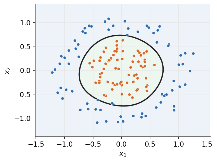
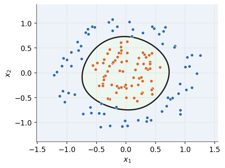
| - | *An RBF kernel separates classes that are not linearly separable, with a nonlinear boundary in the input space.* |
| - | |
| - | ## 7.4 Lagrangian and duality |
| - | |
| - | ### 7.4.1 Lagrangian |
| - | |
| - | For a primal objective $f(w)$ with inequality constraints $g_i(w) \le 0$ and multipliers |
| - | $\beta_i \ge 0$, the Lagrangian is defined as: |
| - | |
| - | $$\boxed{ \mathcal{L}(w,\beta) = f(w) + \sum_{i=1}^{m} \beta_i \, g_i(w) }$$ |
| - | |
| - | Applied to the SVM primal $\tfrac{1}{2}\lVert w \rVert^2$ with constraints |
| - | $1 - y^{(i)}(w^T x^{(i)} - b) \le 0$, the stationarity conditions $\nabla_w \mathcal{L} = 0$ and |
| - | $\partial_b \mathcal{L} = 0$ give: |
| - | |
| - | $$\boxed{ w = \sum_{i=1}^{m} \beta_i\, y^{(i)} x^{(i)}, \qquad \sum_{i=1}^{m} \beta_i\, y^{(i)} = 0 }$$ |
| - | |
| - | So the optimal $w$ is a linear combination of the training inputs weighted by $\beta_i y^{(i)}$. |
| - | |
| - | ### 7.4.2 Dual problem |
| - | |
| - | Substituting these back eliminates $w$ and $b$, leaving a problem in $\beta$ that depends on the |
| - | data only through inner products: |
| - | |
| - | $$\boxed{ \max_{\beta} \ \sum_{i=1}^{m}\beta_i - \tfrac{1}{2}\sum_{i,j}\beta_i \beta_j\, y^{(i)} y^{(j)} \langle x^{(i)}, x^{(j)} \rangle \quad \text{s.t.} \quad \beta_i \ge 0, \ \ \sum_{i}\beta_i y^{(i)} = 0 }$$ |
| - | |
| - | The inner products are exactly where a kernel $K$ is substituted (see [Kernels](/en/Machine%20Learning/07%20Support%20Vector%20Machines#73-kernels)). |
| - | |
| - | ### 7.4.3 KKT and support vectors |
| - | |
| - | At the optimum, complementary slackness ties each multiplier to its constraint: |
| - | |
| - | $$\boxed{ \beta_i \big[\, y^{(i)}(w^T x^{(i)} - b) - 1 \,\big] = 0 }$$ |
| - | |
| - | Support vectors are defined as the examples with a nonzero multiplier: |
| - | |
| - | $$\boxed{ \text{support vectors} = \{\, i : \beta_i > 0 \,\} }$$ |
| - | |
| - | These are the points exactly on the margin. All others have $\beta_i = 0$ and do not affect $w$. |
| - | |
| - | ### 7.4.4 Kernelized decision |
| - | |
| - | Replacing the inner product by a kernel gives a decision rule expressed only through support vectors: |
| - | |
| - | $$\boxed{ h(x) = \operatorname{sign}\!\left( \sum_{i=1}^{m} \beta_i\, y^{(i)}\, K(x^{(i)}, x) - b \right) }$$ |
| - | |
| - | *Remark:* only support vectors ($\beta_i > 0$) contribute, so prediction cost scales with their |
| - | count, not with $m$. |
| - | |
| - | ### 7.4.5 From primal to decision |
| - | |
| - | ```mermaid |
| - | flowchart TD |
| - | A["primal QP: minimize half norm squared"] |
| - | B["Lagrangian with multipliers"] |
| - | C["dual problem in beta"] |
| - | D["KKT conditions"] |
| - | E["support vectors: beta greater than zero"] |
| - | F["kernelized decision rule"] |
| - | A --> B |
| - | B --> C |
| - | C --> D |
| - | D --> E |
| - | E --> F |
| - | ``` |
| - | |
| - | *Support vector machines draw a single, possibly kernelized, boundary. The final part takes a different route: split the feature space with simple rules and combine many such models into an ensemble.* |
| - | |
| - | --- |
| - | Next: [Decision trees and ensemble methods](/en/Machine%20Learning/08%20Decision%20trees%20and%20ensemble%20methods) · [Course overview](/en/Machine%20Learning) |
| en/Machine Learning/07 Support Vector Machines/svm-kernel.png .. /dev/null | |
| en/Machine Learning/07 Support Vector Machines/svm-margin.png .. /dev/null | |
| fr/Machine Learning.md .. | |
| @@ 12,8 12,7 @@ | |
| 4. [Régression linéaire](/fr/Machine%20Learning/04%20Linear%20regression) | |
| 5. [Classification linéaire](/fr/Machine%20Learning/05%20Linear%20classification) | |
| 6. [Réseaux de neurones multi-couches](/fr/Machine%20Learning/06%20Multilayer%20neural%20networks) | |
| - | 7. [Machines à vecteurs de support](/fr/Machine%20Learning/07%20Support%20Vector%20Machines) |
| - | 8. [Arbres de décision et méthodes d'ensemble](/fr/Machine%20Learning/08%20Decision%20trees%20and%20ensemble%20methods) |
| + | 7. [Arbres de décision et méthodes d'ensemble](/fr/Machine%20Learning/07%20Decision%20trees%20and%20ensemble%20methods) |
| --- | |
| [MLOps](/fr/MLOps) · [Accueil](/fr) | |
| fr/Machine Learning/02 General concepts.md .. | |
| @@ 18,7 18,6 @@ | |
| | --- | --- | --- | | |
| | Erreur quadratique | $\tfrac{1}{2}(y-z)^2$ | Régression linéaire | | |
| | Logistique | $\log\!\left(1+\exp(-yz)\right)$ | Régression logistique | | |
| - | | Charnière | $\max(0,\,1-yz)$ | SVM | |
| | Entropie croisée | $-\left[\,y\log\hat{y}+(1-y)\log(1-\hat{y})\,\right]$ | Réseaux de neurones | | |
| *Remarque :* $z$ désigne un score brut tel que $w^T x$, tandis que $\hat{y} \in (0,1)$ désigne une probabilité prédite, l'estimation par le modèle de l'étiquette $y$. La ligne d'entropie croisée prend une probabilité $\hat{y}$, non un score brut. | |
| fr/Machine Learning/05 Linear classification.md .. | |
| @@ 70,7 70,7 @@ | |
|  | |
| - | *Le perceptron trouve un hyperplan séparateur, pas nécessairement celui de marge maximale que la machine à vecteurs de support choisira.* |
| + | *Le perceptron trouve un hyperplan séparateur, pas nécessairement celui de plus grande marge.* |
| ### 5.3.4 Perceptron multiclasse | |
| @@ 94,7 94,7 @@ | |
| Si les données sont linéairement séparables, le perceptron converge en un nombre fini de mises à jour, sinon les poids oscillent indéfiniment. Et comme le critère vaut zéro sur tout hyperplan séparateur, tous comptent comme « optimaux », y compris ceux qui frôlent les données. | |
| - | *Remarque :* trois améliorations corrigent ces limites, et chacune ouvre un module. Une activation et une perte lisses donnent la régression logistique, section suivante. Les marges et les fonctions de base mènent à la [machine à vecteurs de support](/fr/Machine%20Learning/07%20Support%20Vector%20Machines). Empiler les neurones en couches donne les [réseaux de neurones multi-couches](/fr/Machine%20Learning/06%20Multilayer%20neural%20networks), point de départ du cours de Deep Learning. |
| + | *Remarque :* deux améliorations corrigent ces limites, et chacune ouvre un module. Une activation et une perte lisses donnent la régression logistique, section suivante. Empiler les neurones en couches donne les [réseaux de neurones multi-couches](/fr/Machine%20Learning/06%20Multilayer%20neural%20networks), point de départ du cours de Deep Learning. |
| ## 5.4 La régression logistique | |
| @@ 246,7 246,7 @@ | |
| | Mise à jour | $w_j \leftarrow w_j - \alpha \sum_{i=1}^{m}\left(\hat{y}^{(i)} - y^{(i)}\right)x_j^{(i)}$ | | |
| | Multiclasse | softmax $\hat{y}_c = \tfrac{\exp(w_c^T x)}{\sum_{j}\exp(w_j^T x)}$ et l'entropie croisée catégorielle | | |
| - | *Remarque :* lues côte à côte, la mise à jour du perceptron (dans son codage $\{0, 1\}$) et celle de la régression logistique sont la même formule, le résidu fois l'entrée, et seule l'activation change (l'échelon pour le perceptron, la sigmoïde pour la régression logistique, et l'identité de la régression linéaire complète la famille). Le cours de Deep Learning reprend précisément ce fil, en empilant de telles unités en couches. Une perte manque volontairement à ce menu, la charnière $\max(0,\,1 - y\,w^T x)$, qui pénalise les petites marges autant que les erreurs : elle appartient à la [SVM](/fr/Machine%20Learning/07%20Support%20Vector%20Machines). |
| + | *Remarque :* lues côte à côte, la mise à jour du perceptron (dans son codage $\{0, 1\}$) et celle de la régression logistique sont la même formule, le résidu fois l'entrée, et seule l'activation change (l'échelon pour le perceptron, la sigmoïde pour la régression logistique, et l'identité de la régression linéaire complète la famille). Le cours de Deep Learning reprend précisément ce fil, en empilant de telles unités en couches. |
| *Les modèles linéaires étant couverts, le module suivant empile ces briques en réseaux de neurones multi-couches.* | |
| fr/Machine Learning/06 Multilayer neural networks.md .. | |
| @@ 181,7 181,7 @@ | |
| </details> | |
| - | *Ce module est la porte d'entrée du cours de [Deep Learning](/fr/Deep%20Learning), qui reprend l'histoire exactement ici : les fonctions d'activation, les optimiseurs, l'initialisation, la normalisation, la régularisation et les architectures bâties dessus. Le module suivant revient aux modèles linéaires sous un nouvel angle, le classifieur à marge maximale.* |
| + | *Ce module est la porte d'entrée du cours de [Deep Learning](/fr/Deep%20Learning), qui reprend l'histoire exactement ici : les fonctions d'activation, les optimiseurs, l'initialisation, la normalisation, la régularisation et les architectures bâties dessus. Le module suivant change complètement d'outil : les arbres de décision, et les ensembles construits dessus.* |
| --- | |
| - | Suivant : [Machines à vecteurs de support](/fr/Machine%20Learning/07%20Support%20Vector%20Machines) · [Vue d'ensemble du cours](/fr/Machine%20Learning) |
| + | Suivant : [Arbres de décision et méthodes d'ensemble](/fr/Machine%20Learning/07%20Decision%20trees%20and%20ensemble%20methods) · [Vue d'ensemble du cours](/fr/Machine%20Learning) |
| fr/Machine Learning/08 Decision trees and ensemble methods.md .. fr/Machine Learning/07 Decision trees and ensemble methods.md | |
| @@ 1,8 1,8 @@ | |
| - | # 8. Arbres de décision et méthodes d'ensemble |
| + | # 7. Arbres de décision et méthodes d'ensemble |
| Pourquoi faire confiance à un seul modèle quand un comité peut voter ? Ce module construit la boîte à outils des ensembles : le bootstrap et le bagging pour réduire la variance, AdaBoost pour transformer des apprenants faibles en un apprenant fort, les arbres de décision comme apprenant de base favori, et les forêts aléatoires comme la combinaison qui gagne en pratique. | |
| - | ## 8.1 Pourquoi un seul modèle ? |
| + | ## 7.1 Pourquoi un seul modèle ? |
| Chaque module jusqu'ici entraîne un modèle et le garde. Un comité de $M$ modèles est presque toujours meilleur que n'importe lequel de ses membres. La combinaison est une moyenne en régression et un vote majoritaire en classification : | |
| @@ 15,11 15,11 @@ | |
| | Bagging | forte capacité (arbres profonds) | en parallèle, sur données rééchantillonnées | la variance | | |
| | Boosting | faible capacité (souches) | en séquence, sur données repondérées | le biais | | |
| - | ## 8.2 Le bootstrap : moyenner la variance |
| + | ## 7.2 Le bootstrap : moyenner la variance |
| Pourquoi combiner aide-t-il ? Entraînez le même modèle flexible, un polynôme de degré 25, sur 100 ensembles d'entraînement différents et les ajustements individuels divergent violemment. Leur moyenne, elle, épouse la vraie courbe. | |
| - |  |
| + | 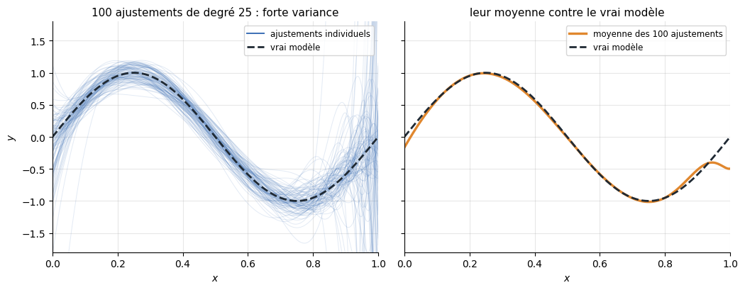 |
| *À gauche : 100 ajustements de degré 25, un par ensemble d'entraînement, chacun poursuivant son propre bruit. À droite : leur moyenne est bien plus proche de la vérité, les fluctuations s'annulent.* | |
| @@ 33,11 33,11 @@ | |
| Le même exemple peut apparaître plusieurs fois dans un rééchantillon, et la probabilité qu'un exemple donné n'apparaisse jamais vaut $(1-\tfrac1N)^N\to e^{-1}\approx0{,}37$ : environ 37 % des données restent hors de chaque rééchantillon. Ce sont ses exemples hors-sac (OOB), que les forêts aléatoires mettront à profit plus bas. | |
| - | ## 8.3 Le bagging |
| + | ## 7.3 Le bagging |
| Le bagging (Bootstrap AGGregating) est le comité construit sur le bootstrap : rééchantillonner $m$ ensembles d'entraînement, entraîner un modèle sur chacun, combiner les votes. | |
| - |  |
| + | 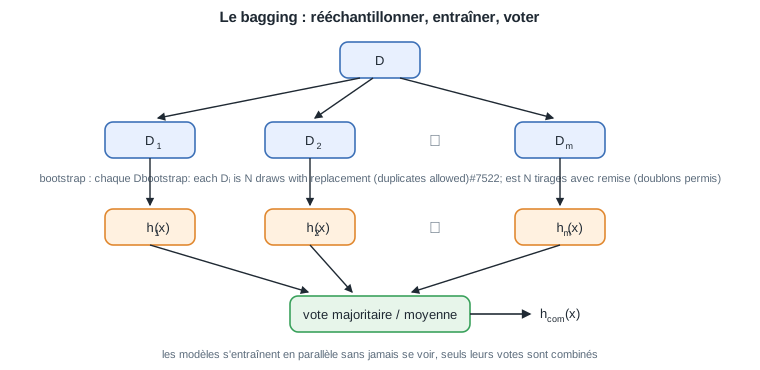 |
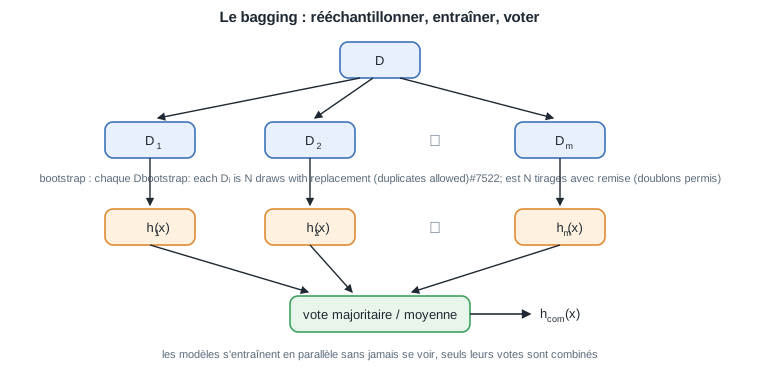
| *Un jeu de données devient $m$ rééchantillons bootstrap, chacun entraîne son propre modèle, et seuls les votes se rencontrent.* | |
| @@ 45,7 45,7 @@ | |
| *Remarque :* moyenner laisse le biais inchangé tout en réduisant la variance, le bagging convient donc aux modèles de base à faible biais et forte variance, exactement les arbres profonds de la section 8.5. Un modèle qui sous-apprend sous-apprend encore après bagging. | |
| - | ## 8.4 Le boosting : AdaBoost |
| + | ## 7.4 Le boosting : AdaBoost |
| Le boosting fait le pari inverse : combiner de nombreux apprenants faibles, à peine meilleurs que le hasard, en un apprenant fort. L'ensemble est une somme pondérée construite un apprenant à la fois : | |
| @@ 57,7 57,7 @@ | |
| 2. Il n'y a **pas de bootstrap** : chaque exemple sert à entraîner chaque apprenant. | |
| 3. Les données sont **repondérées** : les exemples mal classés par $h_t$ gagnent du poids, donc $h_{t+1}$ se concentre sur eux. | |
| - | ### 8.4.1 L'algorithme |
| + | ### 7.4.1 L'algorithme |
| Avec des étiquettes $y\in\{-1,+1\}$, on garde un poids $w^{(i)}$ par exemple, initialisé à $1/N$. À chaque tour $t = 1, \dots, T$ : | |
| @@ 73,13 73,13 @@ | |
| Le classifieur final est le vote pondéré $H_T(x) = \mathrm{sign}\big(\sum_t \alpha_t h_t(x)\big)$. | |
| - |  |
| + | 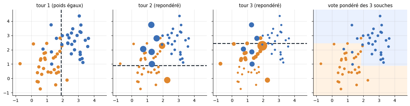 |
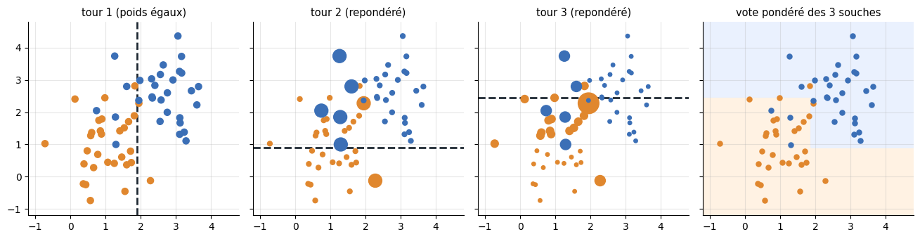
| *Chaque tour ajuste une souche aux données pondérées (taille des points = poids). Les points mal classés gonflent, orientant la souche suivante, et le vote pondéré de trois coupures alignées sur les axes dessine déjà une frontière crénelée, non linéaire.* | |
| *Remarque :* l'apprenant faible classique est la souche (stump), un arbre à une seule coupure perpendiculaire à un axe. Les souches sont très rapides, leur combinaison donne les frontières en escalier ci-dessus, et les $\alpha_t$ appris servent aussi de classement des variables utiles : les variables dont les souches gagnent de grands votes sont les informatives. | |
| - | ### 8.4.2 Gradient boosting |
| + | ### 7.4.2 Gradient boosting |
| Le gradient boosting généralise l'idée à toute perte différentiable $L$. À l'étape $t$, il ajuste l'apprenant suivant sur l'opposé du gradient de la perte évalué au modèle courant, le pseudo-résidu défini par | |
| @@ 98,17 98,17 @@ | |
| | réduit surtout | la variance | le biais | | |
| | repondération | aucune (bootstrap) | poids ou pseudo-résidus | | |
| - | ## 8.5 Arbres de décision |
| + | ## 7.5 Arbres de décision |
| - | ### 8.5.1 Des souches aux arbres |
| + | ### 7.5.1 Des souches aux arbres |
| Une souche pose une question sur une variable. Enchaînez les questions, chaque réponse menant à la souche suivante, et vous obtenez un arbre de décision : une racine, des nœuds internes, et des feuilles qui pavent l'espace d'entrée. | |
| - |  |
| + | 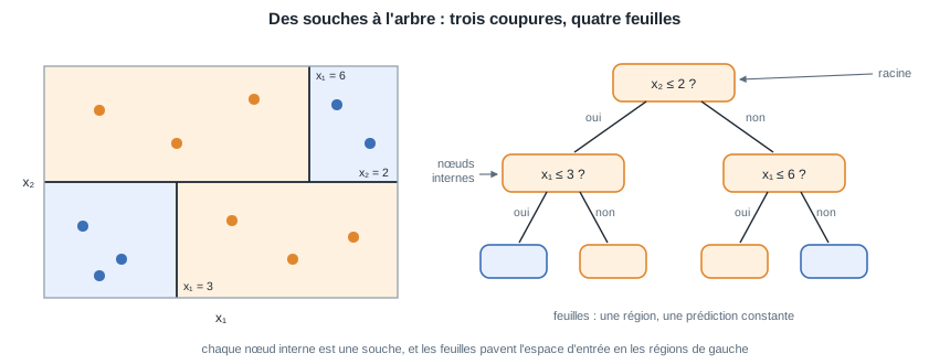 |
| *Trois coupures découpent le plan en quatre régions (à gauche), et les trois mêmes coupures se lisent comme un arbre (à droite) : la racine et les nœuds internes testent des variables, les feuilles prédisent.* | |
| - | ### 8.5.2 L'arbre comme partition |
| + | ### 7.5.2 L'arbre comme partition |
| Un arbre CART partitionne l'espace d'entrée en $M$ régions disjointes $R_1,\dots,R_M$ (les feuilles) et prédit une constante $c_m$ sur chacune. La prédiction est définie par | |
| @@ 118,11 118,11 @@ | |
| *Remarque :* les régions sont des boîtes alignées sur les axes, donc la frontière de décision est en escalier. Un arbre seul a un faible biais mais une forte variance : laissé libre, il coupe jusqu'à isoler chaque valeur aberrante. | |
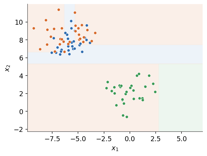
| - |  |
| + |  |
| *Un arbre découpe l'espace en régions alignées sur les axes, chacune à prédiction constante.* | |
| - | ### 8.5.3 Impureté et choix de la coupure |
| + | ### 7.5.3 Impureté et choix de la coupure |
| Quelle question un nœud doit-il poser ? Celle qui laisse les enfants aussi purs que possible. Pour une région de proportions de classes $\hat p_k$, l'impureté mesure le mélange des étiquettes. L'indice de Gini est défini par | |
| @@ 145,7 145,7 @@ | |
| *Remarque :* les deux critères choisissent presque toujours la même coupure. Gini est le défaut de la plupart des implémentations car il évite le logarithme. | |
| - | ### 8.5.4 Arbres de régression |
| + | ### 7.5.4 Arbres de régression |
| En régression, la valeur de la feuille est la moyenne des cibles dans la région, définie par | |
| @@ 153,7 153,7 @@ | |
| et les coupures minimisent l'erreur quadratique intra-région plutôt qu'une impureté de classification. | |
| - | ### 8.5.5 Élagage |
| + | ### 7.5.5 Élagage |
| Un arbre non élagué ajuste exactement l'ensemble d'entraînement et surapprend. L'élagage à complexité coûteuse arbitre entre l'ajustement et la taille de l'arbre $|T|$ (le nombre de feuilles) via une pénalité $\alpha\ge0$ : | |
| @@ 161,7 161,7 @@ | |
| Augmenter $\alpha$ effondre les coupures les plus faibles, produisant une suite emboîtée de sous-arbres. Le meilleur $\alpha$ est choisi par la validation croisée de [Concepts généraux](/fr/Machine%20Learning/02%20General%20concepts). | |
| - | ## 8.6 Forêts aléatoires |
| + | ## 7.6 Forêts aléatoires |
| Une forêt aléatoire est du bagging appliqué à des arbres profonds, plus une seconde source d'aléa. La formule de variance de la section 8.2 disait que le terme résiduel $\rho\sigma^2$ survit à la moyenne, il faut donc décorréler les arbres : à chaque coupure, seul un sous-ensemble aléatoire de $m_{\text{try}}$ variables est considéré comme candidat. Les choix usuels sont | |
| @@ 178,7 178,7 @@ | |
| | corrélation des arbres $\rho$ | plus élevée | plus faible | | |
| | réduction de variance | modérée | plus forte | | |
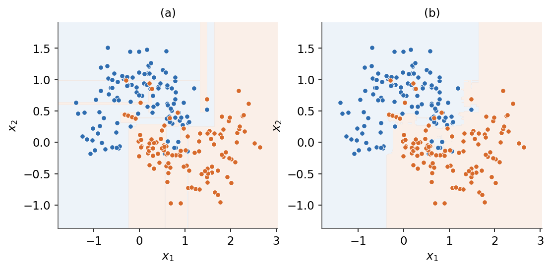
| - |  |
| + |  |
| *(a) Un arbre profond seul surajuste avec une frontière en escalier. (b) Une forêt aléatoire moyenne de nombreux arbres pour une frontière plus lisse.* | |
| fr/Machine Learning/08 Decision trees and ensemble methods/adaboost-rounds.png .. fr/Machine Learning/07 Decision trees and ensemble methods/adaboost-rounds.png | |
| fr/Machine Learning/08 Decision trees and ensemble methods/bagging-pipeline.svg .. fr/Machine Learning/07 Decision trees and ensemble methods/bagging-pipeline.svg | |
| fr/Machine Learning/08 Decision trees and ensemble methods/forest-vs-tree.png .. fr/Machine Learning/07 Decision trees and ensemble methods/forest-vs-tree.png | |
| fr/Machine Learning/08 Decision trees and ensemble methods/tree-boundary.png .. fr/Machine Learning/07 Decision trees and ensemble methods/tree-boundary.png | |
| fr/Machine Learning/08 Decision trees and ensemble methods/tree-from-stumps.svg .. fr/Machine Learning/07 Decision trees and ensemble methods/tree-from-stumps.svg | |
| fr/Machine Learning/08 Decision trees and ensemble methods/variance-reduction.png .. fr/Machine Learning/07 Decision trees and ensemble methods/variance-reduction.png | |
| fr/Machine Learning/07 Support Vector Machines.md .. /dev/null | |
| @@ 1,216 0,0 @@ | |
| - | # 7. Machines à vecteurs de support |
| - | |
| - | Les machines à vecteurs de support sont des classifieurs linéaires à grande marge. Elles |
| - | choisissent la frontière qui maximise la distance aux points les plus proches, contrôlent le |
| - | surapprentissage avec la perte charnière et une pénalité $C$, et utilisent des noyaux pour |
| - | ajuster des frontières non linéaires sans jamais former l'application de caractéristiques. Partout, |
| - | les étiquettes valent $y \in \{-1,+1\}$ et la décision utilise un score brut $z = w^T x - b$. |
| - | |
| - | ## 7.1 Classifieur à marge optimale |
| - | |
| - | Les étiquettes valent $y \in \{-1,+1\}$, avec un vecteur de poids $w \in \mathbb{R}^{n}$ et un biais $b$. |
| - | |
| - | ### 7.1.1 Hypothèse et frontière |
| - | |
| - | L'hypothèse est définie comme le signe du score brut $z = w^T x - b$ : |
| - | |
| - | $$\boxed{ h(x) = \operatorname{sign}(w^T x - b) }$$ |
| - | |
| - | La frontière de décision est l'ensemble des points de score nul : |
| - | |
| - | $$\boxed{ w^T x - b = 0 }$$ |
| - | |
| - | *Remarque :* $w$ est orthogonal à la frontière, il en fixe donc l'orientation, et $b$ fixe le décalage. |
| - | |
| - | ### 7.1.2 Marge géométrique |
| - | |
| - | La marge géométrique de l'exemple $i$ est définie comme sa distance signée à la frontière, rendue |
| - | positive par l'étiquette : |
| - | |
| - | $$\boxed{ \gamma^{(i)} = y^{(i)} \, \frac{w^T x^{(i)} - b}{\lVert w \rVert} }$$ |
| - | |
| - | Un point correctement classé vérifie $\gamma^{(i)} > 0$. La marge du jeu de données est la plus |
| - | petite $\gamma^{(i)}$ sur tous les exemples. |
| - | |
| - | *Remarque :* diviser par $\lVert w \rVert$ rend la marge invariante au rééchelonnement de $(w,b)$, |
| - | contrairement au score brut $z$. |
| - | |
| - | ### 7.1.3 Primal à marge dure |
| - | |
| - | En fixant l'échelle pour que les points les plus proches vérifient $y^{(i)}(w^T x^{(i)} - b) = 1$, |
| - | maximiser la marge équivaut à minimiser $\lVert w \rVert^2$ sous une marge fonctionnelle unitaire : |
| - | |
| - | $$\boxed{ \min_{w,b} \tfrac{1}{2}\lVert w \rVert^2 \quad \text{s.c.} \quad y^{(i)}(w^T x^{(i)} - b) \ge 1 \ \ \forall i }$$ |
| - | |
| - | C'est un programme quadratique convexe à contraintes linéaires, il admet donc un optimum unique. |
| - | |
| - | *Remarque :* il exige des données linéairement séparables. La leçon suivante assouplit cela avec |
| - | des variables d'écart. |
| - | |
| - |  |
| - | |
| - | *L'hyperplan optimal (trait plein) maximise la marge (pointillés). Les points entourés sont les vecteurs de support.* |
| - | |
| - | ## 7.2 Perte charnière |
| - | |
| - | Le score brut est $z = w^T x - b$ et les étiquettes valent $y \in \{-1,+1\}$. |
| - | |
| - | ### 7.2.1 Perte charnière |
| - | |
| - | La perte charnière est définie comme l'écart par lequel la marge $yz$ tombe sous $1$, tronqué à zéro : |
| - | |
| - | $$\boxed{ L(z,y) = \max(0,\, 1 - yz), \quad z = w^T x - b }$$ |
| - | |
| - | Elle est nulle dès que $yz \ge 1$ (le point est correct et au-delà de la marge) et croît |
| - | linéairement à l'intérieur ou au-delà de la marge. |
| - | |
| - | *Remarque :* la perte charnière est convexe mais non dérivable en $yz = 1$, on l'optimise donc |
| - | avec des sous-gradients. |
| - | |
| - | ### 7.2.2 Primal à marge souple |
| - | |
| - | On introduit un écart $\xi_i \ge 0$ par exemple pour autoriser les violations de marge, pénalisé |
| - | par $C > 0$ : |
| - | |
| - | $$\boxed{ \min_{w,b,\xi} \tfrac{1}{2}\lVert w \rVert^2 + C\sum_{i=1}^{m}\xi_i \quad \text{s.c.} \quad y^{(i)}(w^T x^{(i)} - b) \ge 1 - \xi_i, \ \ \xi_i \ge 0 }$$ |
| - | |
| - | À l'optimum $\xi_i = \max(0,\, 1 - y^{(i)}(w^T x^{(i)} - b))$, donc éliminer les écarts donne la |
| - | forme régularisée sans contrainte : |
| - | |
| - | $$\boxed{ \min_{w,b} \tfrac{1}{2}\lVert w \rVert^2 + C\sum_{i=1}^{m}\max\!\big(0,\, 1 - y^{(i)}(w^T x^{(i)} - b)\big) }$$ |
| - | |
| - | C'est de la régularisation plus une perte charnière : le terme $\tfrac{1}{2}\lVert w \rVert^2$ |
| - | élargit la marge et la somme pénalise les violations. |
| - | |
| - | ### 7.2.3 Rôle de $C$ |
| - | |
| - | | $C$ | Pénalité des violations | Marge | Comportement | |
| - | | --- | --- | --- | --- | |
| - | | petit | faible | large | plus de violations tolérées, variance plus faible | |
| - | | grand | forte | étroite | moins de violations, ajuste davantage les données | |
| - | |
| - | *Remarque :* quand $C \to \infty$ aucune violation n'est tolérée, ce qui redonne le classifieur à |
| - | marge dure. |
| - | |
| - | ## 7.3 Noyaux |
| - | |
| - | ### 7.3.1 Définition d'un noyau |
| - | |
| - | Un noyau est défini comme le produit scalaire d'une application de caractéristiques $\phi$ |
| - | appliquée à deux entrées : |
| - | |
| - | $$\boxed{ K(x,z) = \phi(x)^T \phi(z) }$$ |
| - | |
| - | Un noyau valide calcule ce produit scalaire directement, donc $\phi$ n'a jamais à être formée |
| - | (elle peut même être de dimension infinie). |
| - | |
| - | ### 7.3.2 Astuce du noyau |
| - | |
| - | Le dual du SVM ne dépend des données qu'à travers des produits scalaires |
| - | $\langle x^{(i)}, x^{(j)} \rangle$. L'astuce du noyau remplace chaque produit scalaire par un noyau : |
| - | |
| - | $$\boxed{ \langle x^{(i)}, x^{(j)} \rangle \ \longrightarrow \ K(x^{(i)}, x^{(j)}) }$$ |
| - | |
| - | Cela ajuste une frontière linéaire dans l'espace de caractéristiques, donc non linéaire dans |
| - | l'espace d'origine, au prix d'évaluer $K$ au lieu de $\phi$. |
| - | |
| - | Un choix très répandu est le noyau gaussien (RBF) : |
| - | |
| - | $$\boxed{ K(x,z) = \exp\!\left( -\frac{\lVert x - z \rVert^2}{2\sigma^2} \right) }$$ |
| - | |
| - | ### 7.3.3 Condition de Mercer |
| - | |
| - | Une fonction $K$ est un noyau valide si et seulement si, pour tout échantillon fini, sa matrice de |
| - | Gram est symétrique semi-définie positive : |
| - | |
| - | $$\boxed{ K = K^T, \qquad K \succeq 0 }$$ |
| - | |
| - | *Remarque :* c'est la condition de Mercer. Elle garantit l'existence d'une application $\phi$, donc |
| - | le dual reste convexe. |
| - | |
| - | ### 7.3.4 Noyaux usuels |
| - | |
| - | | Noyau | $K(x,z)$ | Note | |
| - | | --- | --- | --- | |
| - | | Linéaire | $x^T z$ | pas d'application, redonne le SVM linéaire | |
| - | | Polynomial | $(x^T z + c)^d$ | degré $d$, décalage $c$ | |
| - | | Gaussien (RBF) | $\exp\!\big(-\tfrac{\lVert x - z \rVert^2}{2\sigma^2}\big)$ | dimension infinie, local | |
| - | |
| - | *Remarque :* un petit $\sigma$ rend le noyau RBF très local, ce qui peut surapprendre. Il se règle |
| - | en compromis avec $C$. |
| - | |
| - |  |
| - | |
| - | *Un noyau RBF sépare des classes non linéairement séparables, par une frontière non linéaire dans l'espace d'entrée.* |
| - | |
| - | ## 7.4 Lagrangien et dualité |
| - | |
| - | ### 7.4.1 Lagrangien |
| - | |
| - | Pour un objectif primal $f(w)$ avec contraintes d'inégalité $g_i(w) \le 0$ et multiplicateurs |
| - | $\beta_i \ge 0$, le lagrangien est défini comme : |
| - | |
| - | $$\boxed{ \mathcal{L}(w,\beta) = f(w) + \sum_{i=1}^{m} \beta_i \, g_i(w) }$$ |
| - | |
| - | Appliqué au primal SVM $\tfrac{1}{2}\lVert w \rVert^2$ avec contraintes |
| - | $1 - y^{(i)}(w^T x^{(i)} - b) \le 0$, les conditions de stationnarité $\nabla_w \mathcal{L} = 0$ et |
| - | $\partial_b \mathcal{L} = 0$ donnent : |
| - | |
| - | $$\boxed{ w = \sum_{i=1}^{m} \beta_i\, y^{(i)} x^{(i)}, \qquad \sum_{i=1}^{m} \beta_i\, y^{(i)} = 0 }$$ |
| - | |
| - | Le $w$ optimal est donc une combinaison linéaire des entrées d'apprentissage pondérées par |
| - | $\beta_i y^{(i)}$. |
| - | |
| - | ### 7.4.2 Problème dual |
| - | |
| - | En réinjectant ces relations, on élimine $w$ et $b$, ce qui laisse un problème en $\beta$ ne |
| - | dépendant des données qu'à travers des produits scalaires : |
| - | |
| - | $$\boxed{ \max_{\beta} \ \sum_{i=1}^{m}\beta_i - \tfrac{1}{2}\sum_{i,j}\beta_i \beta_j\, y^{(i)} y^{(j)} \langle x^{(i)}, x^{(j)} \rangle \quad \text{s.c.} \quad \beta_i \ge 0, \ \ \sum_{i}\beta_i y^{(i)} = 0 }$$ |
| - | |
| - | Les produits scalaires sont exactement l'endroit où l'on substitue un noyau $K$ (voir [Noyaux](/fr/Machine%20Learning/07%20Support%20Vector%20Machines#73-noyaux)). |
| - | |
| - | ### 7.4.3 KKT et vecteurs de support |
| - | |
| - | À l'optimum, l'écart complémentaire lie chaque multiplicateur à sa contrainte : |
| - | |
| - | $$\boxed{ \beta_i \big[\, y^{(i)}(w^T x^{(i)} - b) - 1 \,\big] = 0 }$$ |
| - | |
| - | Les vecteurs de support sont définis comme les exemples à multiplicateur non nul : |
| - | |
| - | $$\boxed{ \text{vecteurs de support} = \{\, i : \beta_i > 0 \,\} }$$ |
| - | |
| - | Ce sont les points exactement sur la marge. Tous les autres ont $\beta_i = 0$ et n'influencent pas |
| - | $w$. |
| - | |
| - | ### 7.4.4 Décision à noyau |
| - | |
| - | Remplacer le produit scalaire par un noyau donne une règle de décision exprimée uniquement à |
| - | travers les vecteurs de support : |
| - | |
| - | $$\boxed{ h(x) = \operatorname{sign}\!\left( \sum_{i=1}^{m} \beta_i\, y^{(i)}\, K(x^{(i)}, x) - b \right) }$$ |
| - | |
| - | *Remarque :* seuls les vecteurs de support ($\beta_i > 0$) contribuent, donc le coût de prédiction |
| - | croît avec leur nombre, pas avec $m$. |
| - | |
| - | ### 7.4.5 Du primal à la décision |
| - | |
| - | ```mermaid |
| - | flowchart TD |
| - | A["QP primal : minimiser demi norme au carre"] |
| - | B["lagrangien avec multiplicateurs"] |
| - | C["probleme dual en beta"] |
| - | D["conditions KKT"] |
| - | E["vecteurs de support : beta superieur a zero"] |
| - | F["regle de decision a noyau"] |
| - | A --> B |
| - | B --> C |
| - | C --> D |
| - | D --> E |
| - | E --> F |
| - | ``` |
| - | |
| - | *Les machines à vecteurs de support tracent une seule frontière, éventuellement à noyau. La dernière partie suit une autre voie : découper l'espace des variables par des règles simples et combiner de nombreux modèles en un ensemble.* |
| - | |
| - | --- |
| - | Suivant : [Arbres de décision et méthodes d'ensemble](/fr/Machine%20Learning/08%20Decision%20trees%20and%20ensemble%20methods) · [Vue d'ensemble du cours](/fr/Machine%20Learning) |
| fr/Machine Learning/07 Support Vector Machines/svm-kernel.png .. /dev/null | |
| fr/Machine Learning/07 Support Vector Machines/svm-margin.png .. /dev/null | |