
5. Linear classification
Classification predicts a discrete label from the same linear score \(w^T x\). This module surveys the classical linear classifiers as one menu: least squares, which assumes Gaussian-shaped classes and admits a closed form, and the perceptron and logistic regression, which assume nothing about the distribution and are fitted by gradient descent. Regularization closes the module.
5.1 The linear separator
A linear classifier assigns the class from the sign of the linear score, and the set of inputs scoring zero is the decision boundary:
\[\boxed{ h_w(x) = \mathrm{sign}(w^T x), \qquad w^T x = 0 \ \text{is the boundary} }\]The boundary is a hyperplane: a line with two features, a plane with three. The sign of the score says on which side of the hyperplane the input falls, and its magnitude how far from the boundary it sits. With \(w = (-4, 1, 2)\) (bias first, on the augmented input), the point \(x = (3, 2)\) scores \(-4 + 3 + 4 = 3\) and falls in front of the hyperplane, while \(x = (1, 1)\) scores \(-4 + 1 + 2 = -1\) and falls behind it.
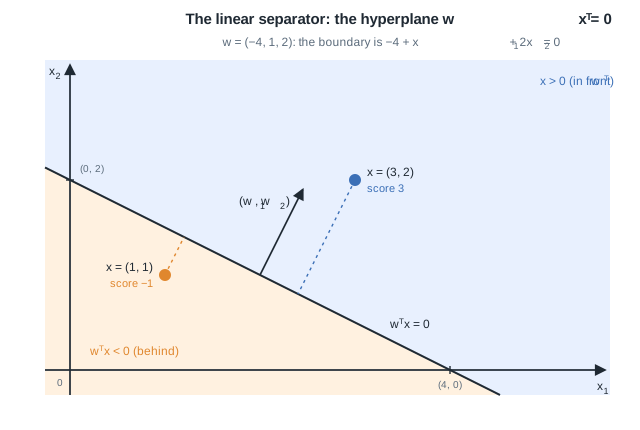
The hyperplane \(w^T x = 0\) splits the input space in two: with \(w = (-4, 1, 2)\) the boundary is the line \(-4 + x_1 + 2x_2 = 0\), normal to \((w_1, w_2)\). The point \((3, 2)\) scores \(3\) and falls in front, \((1, 1)\) scores \(-1\) and falls behind, and the magnitude of the score grows with the distance to the boundary (dotted).
Remark: two practical advantages follow. Once training is done the training set can be thrown away, and predicting costs a single dot product.
5.2 Least squares as a classifier
Code the two classes as \(y \in \{-1, +1\}\), treat them as regression targets, and everything from Linear regression applies verbatim, closed form included:
\[\boxed{ w = (X^T X)^{-1}X^T y, \qquad h_w(x) = \mathrm{sign}(w^T x) }\]For \(K > 2\) classes, code each label as a one-hot row of \(Y \in \mathbb{R}^{m \times K}\) and reuse the multiple-output regression of Linear regression, predicting the class with the highest score:
\[\boxed{ W = (X^T X)^{-1}X^T Y, \qquad \hat{y} = \arg\max_k \; (W^T x)_k }\]It can work, but the squared loss penalizes large scores even deep on the correct side, so the points least in doubt pull on the boundary. That is the Gaussian assumption at work: least squares treats the labels as Gaussian targets, and data far from that story breaks it.
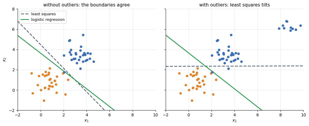
Without outliers least squares and logistic regression agree. Adding distant, correctly classified points tilts the least-squares boundary into errors, while logistic regression barely moves.
5.3 The perceptron
5.3.1 The model: one neuron
The first assumption-free method takes the definition of a linear classifier at face value, a dot product followed by a hard activation, the historical neuron:
\[\boxed{ h_w(x) = \mathrm{sign}(w^T x), \qquad y \in \{-1, +1\} }\]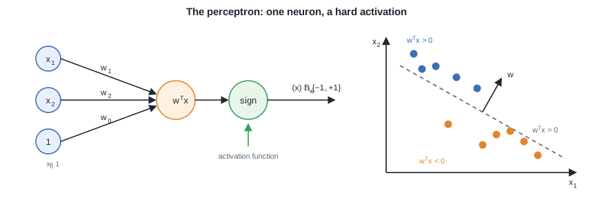
Left: the perceptron is a single neuron, the weighted inputs summed into the score \(w^T x\) and passed through a hard sign activation. Right: that sign splits the input space along the hyperplane \(w^T x = 0\).
5.3.2 The loss function: the perceptron criterion
Fitting needs a loss, and counting mistakes does not work: the count is piecewise constant, so its gradient is zero almost everywhere. The perceptron criterion instead penalizes each misclassified point by how far it sits on the wrong side. A mistake means \(y^{(i)}\,w^T x^{(i)} < 0\), so over the set \(\mathcal{M}\) of misclassified points:
\[\boxed{ E(w) = -\sum_{i \in \mathcal{M}} y^{(i)}\, w^T x^{(i)} }\]always positive and piecewise linear.
5.3.3 Optimization: gradient descent
Minimizing the criterion introduces the workhorse of everything in this course that lacks a closed form, gradient descent: repeatedly step the parameters against the gradient of the loss, scaled by a learning rate \(\alpha > 0\):
\[\boxed{\,w \leftarrow w - \alpha\,\nabla_w E(w)\,}\]The batch variant computes the gradient over the whole training set before each step, a smooth descent that reads every example every time. The stochastic variant (SGD) steps on one example at a time, cheap and noisy, and is the default on large datasets. If \(\alpha\) is too large the iterates can diverge, if too small convergence crawls.
Remark: fancier optimizers exist, momentum, Adam and their cousins, refinements of this same rule that matter for deep networks (Optimization in the Deep Learning course). Everything in this module needs only the plain version.
On a single misclassified example the gradient of the criterion is \(-y^{(i)} x^{(i)}\), so the stochastic step is the perceptron update: on a mistake,
\[\boxed{ w \leftarrow w + \alpha\, y^{(i)} x^{(i)} }\]and no update otherwise. In the \(\{0, 1\}\) coding this is the residual-times-input update \(w_j \leftarrow w_j + \alpha\,(y^{(i)} - h_w(x^{(i)}))\,x_j^{(i)}\).
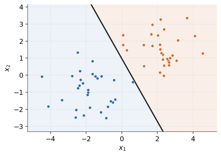
The perceptron finds one separating hyperplane, not necessarily the maximum-margin one the support vector machine will choose.
5.3.4 Multiclass perceptron
With \(k\) classes, keep one weight vector \(w_c\) per class and predict the highest-scoring one. On a mistake, reward the true class and penalize the predicted one:
\[\boxed{ \hat{y} = \arg\max_c w_c^T x, \qquad w_{y} \mathrel{+}= \alpha x, \quad w_{\hat{y}} \mathrel{-}= \alpha x }\]The network view extends naturally: one score neuron per class, and an argmax where the binary perceptron had a sign. Gathering the \(w_c\) as the columns of a matrix \(W \in \mathbb{R}^{(n+1) \times k}\), one product \(W^T x\) computes every score at once, and the scores carve the input space into \(k\) regions, each claimed by the class whose score is largest.
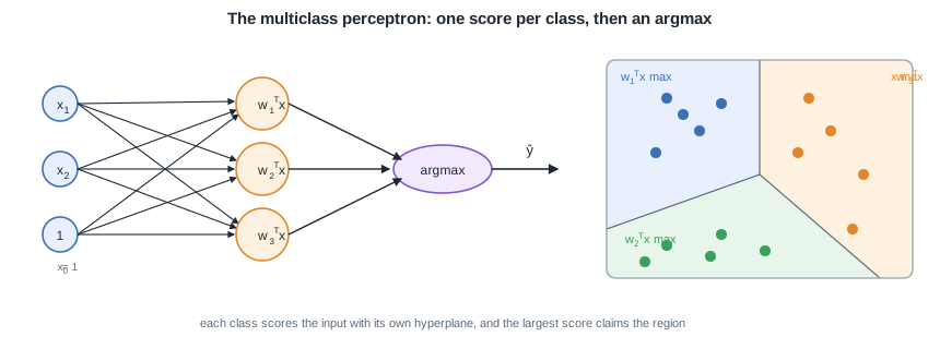
One score neuron per class and an argmax on top. Each column of \(W\) (each row of \(W^T\)) is the hyperplane, normal and bias, of one class.
A worked example with \(k = 3\) classes and the input \(x = (1.1, -2.0)\), augmented with \(x_0 = 1\):
\[ W^T x = \begin{bmatrix} -2 & -4 & 1 \\ -4 & 2 & 4 \\ -6 & 4 & -5 \end{bmatrix}\begin{bmatrix} 1 \\ 1.1 \\ -2.0 \end{bmatrix} = \begin{bmatrix} -8.4 \\ -9.8 \\ 8.4 \end{bmatrix} \]The third score wins, so the input is assigned to class 3. Reading off the third row, that score is \(w_3^T x = -6 + 4 \times 1.1 + (-5) \times (-2.0) = 8.4\).
5.3.5 Convergence and limits
If the data is linearly separable the perceptron converges in a finite number of updates, otherwise the weights oscillate forever. And since the criterion is zero on every separating hyperplane, all of them count as "optimal", including those that graze the data.
Remark: three upgrades fix these limits, and each one opens a module. A smooth activation and loss give logistic regression, next section. Margins and basis functions lead to the Support Vector Machine. Stacking neurons into layers gives multilayer neural networks, the starting point of the Deep Learning course.
5.4 Logistic regression
5.4.1 The model: a smooth activation
Logistic regression keeps the neuron but replaces the hard step with the smooth sigmoid, so the output is the probability of the positive class (\(y \in \{0, 1\}\)). It is still written \(\hat{y}\), but the estimate of the label is now soft: the perceptron's \(\hat{y}\) was a hard class, logistic regression's is a probability, and thresholding it at \(\tfrac{1}{2}\) turns it back into a class whenever one is needed:
\[\boxed{ \hat{y} = p(y = 1 \mid x; w) = \sigma(w^T x) = \frac{1}{1 + e^{-w^T x}} }\]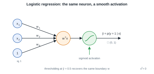
The same neuron with the step swapped for the sigmoid: the output becomes the probability \(\hat{y} = p(y = 1 \mid x)\), and thresholding it at \(\tfrac{1}{2}\) recovers the same boundary \(w^T x = 0\).
Remark: the sigmoid is not an arbitrary squashing choice. Writing the posterior with Bayes' rule gives \(p(C_1 \mid x) = 1/(1 + e^{-a})\) with \(a = \ln \frac{p(x \mid C_1)\,p(C_1)}{p(x \mid C_0)\,p(C_0)}\), so a well-trained logistic output is exactly a posterior probability.
5.4.2 The loss function: cross-entropy
The likelihood of Bernoulli labels, taken through \(-\log\), gives the cross-entropy loss:
\[\boxed{ L(w) = -\sum_{i=1}^{m}\left[ y^{(i)}\log \hat{y}^{(i)} + (1 - y^{(i)})\log(1 - \hat{y}^{(i)}) \right] }\]Proof: maximum likelihood gives the cross-entropy
The model says each label is a Bernoulli draw with success probability \(\hat{y}^{(i)} = \sigma(w^T x^{(i)})\), and both cases fold into one expression:
\[p(y^{(i)} \mid x^{(i)}; w) = \left(\hat{y}^{(i)}\right)^{y^{(i)}}\left(1 - \hat{y}^{(i)}\right)^{1 - y^{(i)}}\]since \(y^{(i)} \in \{0, 1\}\) selects the factor: the expression is \(\hat{y}^{(i)}\) when \(y^{(i)} = 1\) and \(1 - \hat{y}^{(i)}\) when \(y^{(i)} = 0\). The examples are i.i.d., so the likelihood of the training set factorizes, as it did in Linear regression:
\[p(y \mid X; w) = \prod_{i=1}^{m} \left(\hat{y}^{(i)}\right)^{y^{(i)}}\left(1 - \hat{y}^{(i)}\right)^{1 - y^{(i)}}\]The logarithm preserves the argmax, turns the product into a sum and brings the exponents down:
\[\ell(w) = \sum_{i=1}^{m}\left[ y^{(i)}\log \hat{y}^{(i)} + (1 - y^{(i)})\log(1 - \hat{y}^{(i)}) \right]\]Maximizing \(\ell\) is minimizing \(-\ell\), which is exactly \(L(w)\). The cross-entropy is the negative Bernoulli log-likelihood, the same estimation principle that made least squares the answer under Gaussian noise. \(\blacksquare\)
5.4.3 Optimization: gradient descent
Unlike least squares, this loss has no closed-form minimizer: the sigmoid makes the stationarity equations transcendental, so the fit falls to the same gradient descent as the perceptron. Differentiating the cross-entropy through the sigmoid rewards the effort: almost everything cancels and the gradient collapses to the residual times the input:
\[\boxed{ w_j \leftarrow w_j - \alpha \sum_{i=1}^{m}\left(\hat{y}^{(i)} - y^{(i)}\right)x_j^{(i)} }\]Proof: the gradient collapses to the residual times the input
Write the score \(z^{(i)} = w^T x^{(i)}\), so that \(\hat{y}^{(i)} = \sigma(z^{(i)})\). The derivation rests on one identity, the sigmoid differentiating into itself:
\[\sigma'(z) = \frac{e^{-z}}{\left(1 + e^{-z}\right)^2} = \frac{1}{1 + e^{-z}} \cdot \frac{e^{-z}}{1 + e^{-z}} = \sigma(z)\left(1 - \sigma(z)\right)\]since \(\tfrac{e^{-z}}{1 + e^{-z}} = 1 - \sigma(z)\). Now take the loss of a single example, \(L^{(i)} = -\left[y^{(i)}\log \hat{y}^{(i)} + (1 - y^{(i)})\log(1 - \hat{y}^{(i)})\right]\), and follow the chain rule through its three stages, loss to output, output to score, score to weight:
\[\frac{\partial L^{(i)}}{\partial \hat{y}^{(i)}} = -\frac{y^{(i)}}{\hat{y}^{(i)}} + \frac{1 - y^{(i)}}{1 - \hat{y}^{(i)}} = \frac{\hat{y}^{(i)} - y^{(i)}}{\hat{y}^{(i)}\left(1 - \hat{y}^{(i)}\right)}, \qquad \frac{\partial \hat{y}^{(i)}}{\partial z^{(i)}} = \hat{y}^{(i)}\left(1 - \hat{y}^{(i)}\right), \qquad \frac{\partial z^{(i)}}{\partial w_j} = x_j^{(i)}\](the first equality puts the two fractions over the common denominator \(\hat{y}^{(i)}(1 - \hat{y}^{(i)})\), and the second is the sigmoid identity above). Multiplying the three, the denominator of the first factor is exactly the second factor, and everything cancels:
\[\frac{\partial L^{(i)}}{\partial w_j} = \frac{\hat{y}^{(i)} - y^{(i)}}{\hat{y}^{(i)}\left(1 - \hat{y}^{(i)}\right)} \cdot \hat{y}^{(i)}\left(1 - \hat{y}^{(i)}\right) \cdot x_j^{(i)} = \left(\hat{y}^{(i)} - y^{(i)}\right) x_j^{(i)}\]Summing over the training set gives \(\partial L / \partial w_j = \sum_{i=1}^{m} (\hat{y}^{(i)} - y^{(i)})\, x_j^{(i)}\), and plugging this gradient into the descent rule \(w \leftarrow w - \alpha\, \nabla_w L\) is the boxed update. \(\blacksquare\)
Remark: unlike the perceptron, the gradient involves every training point, not only the misclassified ones: each point pulls in proportion to its residual \(\hat{y}^{(i)} - y^{(i)}\). That is what makes logistic regression more stable than the perceptron and usable on non-separable data.
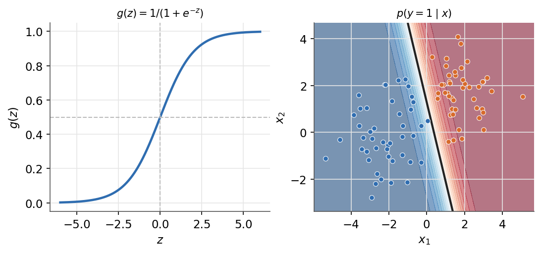
Left: the sigmoid maps any score into the interval (0, 1). Right: the decision boundary and the predicted probability.
5.4.4 Multiclass: the softmax
For \(k\) classes the sigmoid generalizes to the softmax: one weight vector \(w_c\), hence one score, per class, exponentials that make the scores positive, and a normalization that turns them into a distribution. Writing \(\hat{y}_c\) for the predicted probability of class \(c\), as \(\hat{y}\) was the probability of the positive class above:
\[\boxed{ \hat{y}_c = p(y = c \mid x; w) = \frac{\exp(w_c^T x)}{\sum_{j=1}^{k}\exp(w_j^T x)} }\]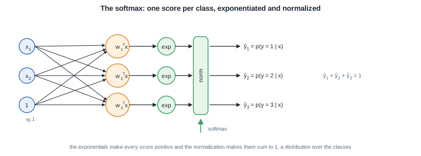
The multiclass network with a softmax head: each class scores the input, the exponentials make the scores positive, and the normalization turns them into probabilities that sum to 1. It is the multiclass perceptron's network with the argmax replaced by a smooth, differentiable head.
With one-hot labels the loss is the categorical cross-entropy \(L = -\sum_i \log p(y^{(i)} \mid x^{(i)})\), whose gradient keeps the same residual-times-input form.
| sigmoid | softmax | |
|---|---|---|
| classes | 2 | \(k\) |
| output | one probability \(\hat{y}\) | a distribution over \(k\) classes |
| relation | the \(k = 2\) softmax reduces to the sigmoid | generalizes the sigmoid |
Proof: the softmax at k = 2 is the sigmoid
With two classes the softmax scores the input twice, \(w_1\) for the positive class and \(w_0\) for the negative one:
\[p(y = 1 \mid x; w) = \frac{e^{w_1^T x}}{e^{w_1^T x} + e^{w_0^T x}}\]Dividing numerator and denominator by \(e^{w_1^T x}\) leaves
\[p(y = 1 \mid x; w) = \frac{1}{1 + e^{-(w_1 - w_0)^T x}} = \sigma\!\left((w_1 - w_0)^T x\right)\]the sigmoid applied to the difference of the scores. Only the difference \(w = w_1 - w_0\) matters (the general fact behind this: shifting every \(w_c\) by the same vector leaves the softmax unchanged), so a single weight vector suffices, exactly the binary model this section started from. Read in the other direction, this is the recipe for the generalization: give each class its own score \(w_c^T x\), exponentiate to make the scores positive, normalize so they sum to one, and the two-class case collapses back to one sigmoid. \(\blacksquare\)
5.5 Regularized classification
Nothing pins down the scale of \(w\): doubling it moves no perceptron boundary and only sharpens the probabilities of logistic regression, and different weight vectors can produce identical scores. The maximum a posteriori recipe of Linear regression applies verbatim, adding a penalty to whichever loss is being minimized:
\[\boxed{ J_\lambda(w) = \sum_{i=1}^{m} L\!\left(h_w(x^{(i)}),\,y^{(i)}\right) + \lambda\,\Omega(w), \qquad \Omega(w) = \lVert w \rVert_2^2 \ \text{or} \ \lVert w \rVert_1 }\]For the cross-entropy with the L2 penalty, the gradient simply gains a pull toward zero, \(\sum_i (\hat{y}^{(i)} - y^{(i)})\,x^{(i)} + 2\lambda w\).
Remark: libraries expose exactly this menu, a loss plus a penalty (scikit-learn's SGDClassifier takes a loss and a penalty argument). The strength \(\lambda\) is chosen by the validation of General concepts, and the lasso's selecting behaviour is covered in Linear regression.
5.6 Summary
The classical methods all fit the same hyperplane, and they split cleanly by what they assume about the data and how they are solved: least squares inherits the closed-form comfort of Linear regression and pays for it with a distributional assumption, the perceptron and logistic regression assume nothing and pay with iterative optimization. Algorithm by algorithm, the formulas that define each one:
Least squares, the one with an assumption and a closed form:
| Formula | |
|---|---|
| Assumption on the data | Gaussian-shaped classes |
| Activation | identity to train (regression on \(\pm 1\) targets), then \(\mathrm{sign}(w^T x)\) to predict |
| Loss | squared error \(\sum_{i=1}^{m}\left(w^T x^{(i)} - y^{(i)}\right)^2\) |
| Fit | closed form \(w = (X^T X)^{-1}X^T y\), no iteration |
| Multiclass | one-hot rows of \(Y\), \(W = (X^T X)^{-1}X^T Y\), predict \(\arg\max_k\,(W^T x)_k\) |
The perceptron, mistake-driven and assumption-free:
| Formula | |
|---|---|
| Assumption on the data | none |
| Activation | step, \(h_w(x) = \mathrm{sign}(w^T x)\), \(y \in \{-1, +1\}\) |
| Loss | perceptron criterion \(E(w) = -\sum_{i \in \mathcal{M}} y^{(i)}\, w^T x^{(i)}\), misclassified points only |
| Gradient | \(\nabla_w E = -\sum_{i \in \mathcal{M}} y^{(i)} x^{(i)}\) |
| Update | \(w \leftarrow w + \alpha\, y^{(i)} x^{(i)}\) on a mistake, nothing otherwise |
| Multiclass | \(\hat{y} = \arg\max_c\, w_c^T x\), then \(w_{y} \mathrel{+}= \alpha x\) and \(w_{\hat{y}} \mathrel{-}= \alpha x\) |
| Convergence | finite if the data is separable, oscillates otherwise |
Logistic regression, probabilistic and assumption-free:
| Formula | |
|---|---|
| Assumption on the data | none |
| Activation | sigmoid, \(\hat{y} = \sigma(w^T x) = \tfrac{1}{1 + e^{-w^T x}}\), a probability, \(y \in \{0, 1\}\) |
| Loss | cross-entropy \(L(w) = -\sum_{i=1}^{m}\left[ y^{(i)}\log \hat{y}^{(i)} + (1 - y^{(i)})\log(1 - \hat{y}^{(i)}) \right]\) |
| Gradient | \(\nabla_{w_j} L = \sum_{i=1}^{m}\left(\hat{y}^{(i)} - y^{(i)}\right)x_j^{(i)}\), every point pulls by its residual |
| Update | \(w_j \leftarrow w_j - \alpha \sum_{i=1}^{m}\left(\hat{y}^{(i)} - y^{(i)}\right)x_j^{(i)}\) |
| Multiclass | softmax \(\hat{y}_c = \tfrac{\exp(w_c^T x)}{\sum_{j}\exp(w_j^T x)}\) and the categorical cross-entropy |
Remark: read side by side, the perceptron update (in its \(\{0, 1\}\) coding) and the logistic update are the same formula, the residual times the input, and only the activation changes (the step for the perceptron, the sigmoid for logistic regression, and the identity of linear regression completes the family). The Deep Learning course picks up exactly this thread, stacking such units into layers. One loss is deliberately missing from this menu, the hinge \(\max(0,\,1 - y\,w^T x)\), which penalizes small margins as well as mistakes: it belongs to the SVM.
With linear models covered, the next module stacks these building blocks into multilayer neural networks.