
# 10. Transformers The Transformer replaces recurrence with attention alone. It processes a whole sequence of token embeddings in parallel, letting every token attend to every other token through learned queries, keys, and values. This lesson builds the architecture from self-attention, assuming embeddings (lesson 6) and the attention mechanism (lesson 9), and reuses normalization (lesson 4) and residual connections (lesson 5). ## 10.1 Self-attention and Q, K, V A sequence of $n$ tokens is represented by an embedding matrix $X \in \mathbb{R}^{n \times d}$, one row per token. Self-attention lets each token gather information from the others by asking a question (a query), matching it against every token's label (a key), and reading out content (a value). From the same input $X$ we form three projections with learned matrices $W^Q, W^K \in \mathbb{R}^{d \times d_k}$ and $W^V \in \mathbb{R}^{d \times d_v}$: $$\boxed{ Q = X W^Q, \quad K = X W^K, \quad V = X W^V }$$ *Remark:* the projections are the only learned parameters here, and the same three matrices are shared across all positions. Because a token is compared against every other token, the operation captures long-range dependencies in a single step, unlike a recurrence that must carry information forward one position at a time. 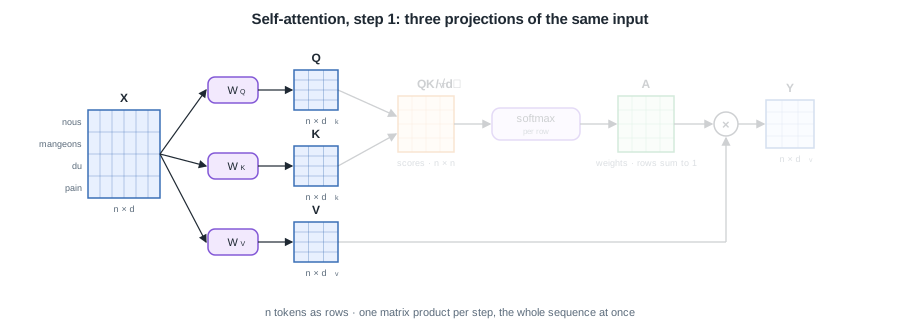 *From one input matrix (here four tokens, "nous mangeons du pain"), three learned projections give every token its query, key, and value. What they feed is still grayed out.* ## 10.2 Scaled dot-product attention Each query is compared against every key by a dot product, giving an $n \times n$ matrix of raw scores. The scores are scaled, turned into weights by a row-wise softmax, and used to average the values: $$\boxed{ \mathrm{Attention}(Q, K, V) = \mathrm{softmax}\!\left( \frac{Q K^{T}}{\sqrt{d_k}} \right) V }$$ Row $i$ of the softmax is a probability distribution over all tokens, so output row $i$ is a weighted average of the value vectors, weighted by how relevant each token is to token $i$. 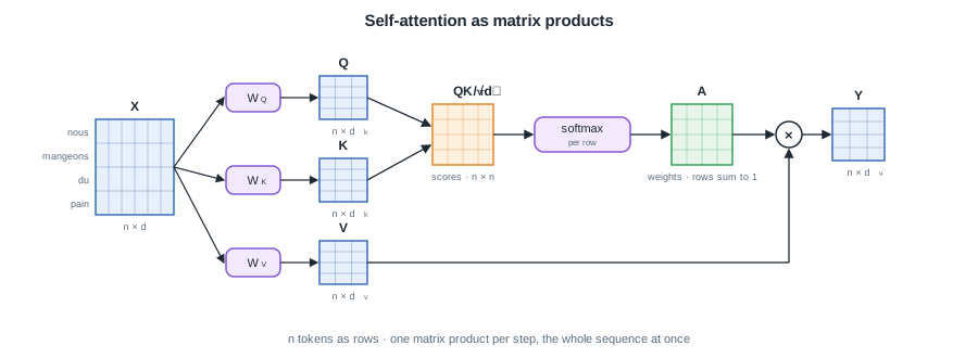 *The whole layer as matrix products, shapes included: $QK^T/\sqrt{d_k}$ compares every token with every other ($n \times n$), the row-wise softmax turns scores into weights, and multiplying by $V$ returns one output row per token.* ### 10.2.1 Why divide by $\sqrt{d_k}$ If the entries of $q$ and $k$ are independent with zero mean and unit variance, the dot product $q^{T} k = \sum_{j=1}^{d_k} q_j k_j$ has variance $d_k$, so its typical magnitude grows like $\sqrt{d_k}$. $$\boxed{ \mathrm{Var}\!\left(q^{T} k\right) = d_k \quad\Rightarrow\quad \frac{q^{T} k}{\sqrt{d_k}} \text{ has unit variance} }$$ Large scores push the softmax into a saturated regime where one weight is near $1$ and the rest are near $0$, and the softmax gradient there is tiny. Dividing by $\sqrt{d_k}$ keeps the logits at a moderate scale, which keeps the softmax gradients healthy and stabilizes training. 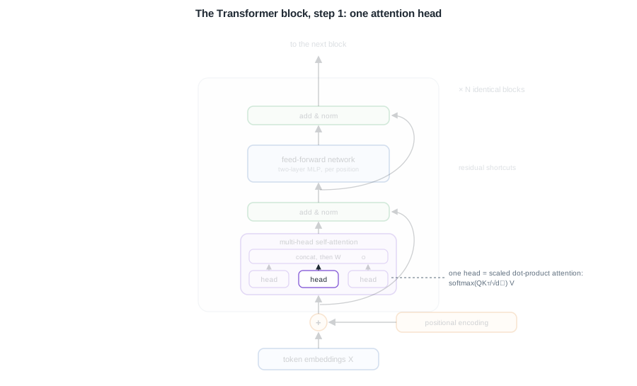 *The unit so far: one scaled dot-product attention head, sitting where it will live. The rest of the block is still grayed out.* ## 10.3 Multi-head attention A single attention computation forces every relationship to be read through one $d_k$-dimensional subspace. Multi-head attention runs $h$ attention operations in parallel, each with its own projections, so different heads can specialize (one on syntax, another on coreference, and so on). Head $i$ projects the inputs with its own matrices $W_i^{Q}, W_i^{K}, W_i^{V}$ and applies scaled dot-product attention: $$\boxed{ \mathrm{head}_i = \mathrm{Attention}\!\left(Q W_i^{Q}, K W_i^{K}, V W_i^{V}\right) }$$ The heads are concatenated along the feature axis and mixed by an output projection $W^{O}$: $$\boxed{ \mathrm{MultiHead}(Q, K, V) = \mathrm{Concat}(\mathrm{head}_1, \dots, \mathrm{head}_h)\, W^{O} }$$ *Remark:* the per-head width is usually set to $d_k = d_v = d / h$, so the concatenation returns to width $d$ and the total cost matches a single full-width head. The heads are independent and computed in parallel, which is one reason Transformers train efficiently on modern hardware. 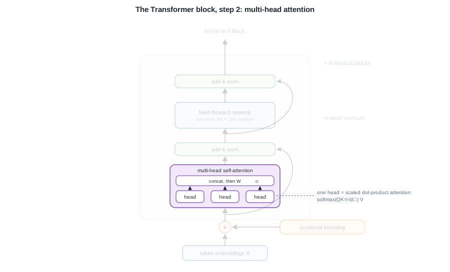 *Step 2: several heads run in parallel on their own projections, and their outputs are concatenated and mixed by $W^O$. The multi-head sublayer is complete.* ## 10.4 Positional encoding Attention treats its input as a set: permuting the rows of $X$ permutes the output the same way, so the operation is order-agnostic. Language is not, therefore position must be supplied explicitly. The original Transformer adds a fixed sinusoidal encoding to the embeddings, using a different frequency per feature dimension: $$\boxed{ PE_{(pos,\, 2i)} = \sin\!\left(\frac{pos}{10000^{2i/d}}\right), \quad PE_{(pos,\, 2i+1)} = \cos\!\left(\frac{pos}{10000^{2i/d}}\right) }$$ Here $pos$ is the token position and $i$ indexes the feature dimension. Low dimensions vary quickly with position and high dimensions vary slowly, so the vector encodes position across many scales. The encoding is added to the token embedding before the first block. 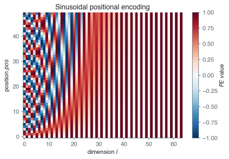 *Sinusoidal positional encodings vary quickly in low dimensions and slowly in high dimensions, giving each position a unique multi-scale signature.* *Remark:* sinusoids let a relative shift $PE_{pos+k}$ be written as a linear function of $PE_{pos}$, so the model can learn to attend by relative offset. The encodings are fixed (not learned) and extend to sequence lengths unseen during training. Many later models replace them with learned or relative position schemes. 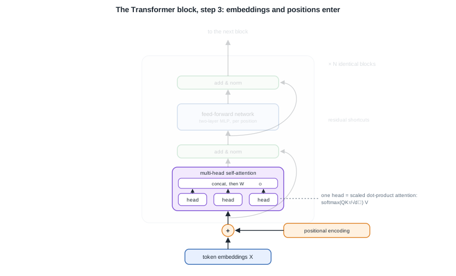 *Step 3: the input side. Token embeddings enter through an addition with the positional encoding, which gives attention its sense of order.* ## 10.5 The Transformer block Each sublayer is wrapped in a residual connection followed by layer normalization, which keeps gradients flowing through deep stacks and stabilizes the activation scale: $$\boxed{ x \leftarrow \mathrm{LayerNorm}\!\left(x + \mathrm{Sublayer}(x)\right) }$$ 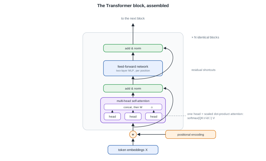 *The assembled block: multi-head self-attention, then the position-wise feed-forward network, each wrapped in a residual connection and layer normalization. Stacked $N$ times, this is the Transformer.* A block chains two sublayers in this pattern. The first is multi-head self-attention (tokens exchange information). The second is a position-wise feed-forward network, a two-layer MLP applied independently to each position, using the notation of lesson 1: $$\boxed{ \mathrm{FFN}(x) = g\!\left(x W_1 + b_1\right) W_2 + b_2 }$$ with a nonlinearity $g$ (ReLU or GELU) and an inner width several times larger than $d$. *Remark:* the residual reuses the identity shortcut of lesson 5, so the sublayer only has to learn a correction to its input. Layer normalization (lesson 4) normalizes across the feature dimension per token, which suits variable-length sequences better than batch normalization. The form above is the original post-norm placement. Many modern implementations use pre-norm, $x \leftarrow x + \mathrm{Sublayer}(\mathrm{LayerNorm}(x))$, which trains more stably at great depth. | Component | Role | Acts across | | --- | --- | --- | | Multi-head attention | mix information between tokens | the sequence | | Feed-forward network | transform each token nonlinearly | the features | | Residual connection | preserve a gradient path | the depth | | Layer normalization | stabilize the activation scale | the features per token | ## 10.6 The encoder-decoder architecture The full Transformer stacks $N$ identical blocks in an encoder and $N$ in a decoder. The encoder maps the input sequence to a set of context vectors. Each decoder block has three sublayers: masked self-attention over the tokens generated so far (the mask blocks attention to future positions), cross-attention whose queries come from the decoder and whose keys and values come from the encoder output, and a feed-forward network. A final linear layer plus softmax turns the top decoder states into a distribution over the vocabulary. 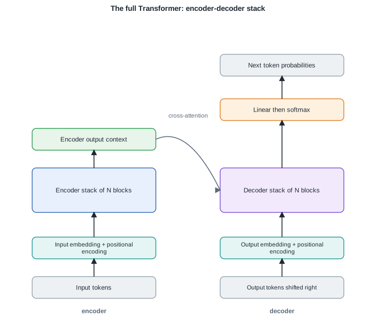 *The full Transformer: a stack of encoder blocks and a stack of decoder blocks joined by cross-attention.* ### 10.6.1 Variants Not every task needs both halves. Two families dominate practice: | Variant | Structure | Attention | Typical use | | --- | --- | --- | --- | | Encoder-only (BERT) | encoder stack | bidirectional | understanding, classification, embeddings | | Decoder-only (GPT) | decoder stack | masked (causal) | generation, autoregressive prediction | | Encoder-decoder (T5) | both stacks | bidirectional plus masked | translation, summarization | *Remark:* an encoder-only model sees the whole sequence at once, which suits labelling and retrieval. A decoder-only model masks the future so it can predict the next token, which is exactly the setup for text generation. *With attention and the Transformer in hand, the arc of this course is complete: from a single perceptron to the architecture behind today's foundation models. To take a trained model from a notebook to a reliable production service, continue with the [MLOps](/en/MLOps) course.* --- Next: [Course overview](/en/Deep%20Learning)