
9. Attention
Recurrent encoder-decoder models push a whole input sequence through a single fixed context vector, which caps how much they can remember for long inputs. Attention removes that bottleneck by letting the decoder read every encoder state directly, weighting each one by how relevant it is to the current output step. This lesson builds the mechanism from alignment scores to the query-key-value view, which is the foundation the Transformer will generalize.
9.1 The seq2seq bottleneck
Take a running example: translating the French "nous mangeons du pain" into "we are eating bread". A sequence-to-sequence model uses an encoder recurrent network to read the input tokens \(x_1, \dots, x_T\) into hidden states \(h_1, \dots, h_T\), then a decoder recurrent network to emit the output tokens, one per step. In the vanilla design the decoder is initialised from a single context vector, the encoder's last hidden state:
\[\boxed{ c = h_T }\]Every decoder step \(i\) produces its state \(s_i\) and its output from this one vector \(c\) plus the previous output. The whole meaning of the input, however long, has to be squeezed into a single fixed-size \(h_T\).
Remark: this is a genuine information bottleneck. For a short sentence \(h_T\) can hold enough, but as \(T\) grows the early tokens are overwritten and translation or summarisation quality drops sharply on long inputs.
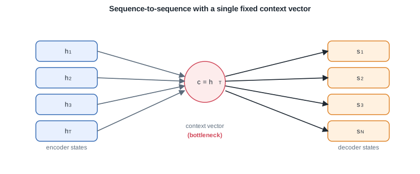
Plain sequence-to-sequence squeezes the whole input into one fixed context vector, a bottleneck for long sequences.
The fix is to keep all encoder states \(h_1, \dots, h_T\) available and let the decoder decide, at each step, which of them to read.
9.2 The attention mechanism
Instead of one context vector shared across all steps, attention builds a fresh context vector \(c_i\) for each decoder step \(i\). It does this in three stages: score, normalise, combine.
9.2.1 Alignment scores
For decoder step \(i\) with state \(s_i\), a score function measures how well that state aligns with each encoder state \(h_j\):
\[e_{i,j} = \operatorname{score}(s_i, h_j)\]A high \(e_{i,j}\) means encoder position \(j\) is relevant to producing output \(i\). The scores form a vector over the \(T\) input positions.
Remark: \(s_i\) is usually the decoder state just before emitting token \(i\), so the model chooses what to look at using what it has produced so far.
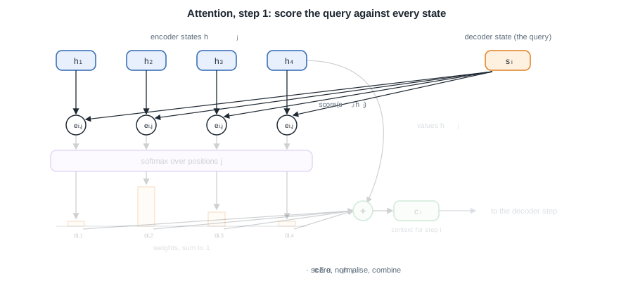
Step 1: the decoder state \(s_i\) is scored against every encoder state \(h_j\), one score per input position. Everything downstream is still grayed out.
9.2.2 Attention weights
The scores are turned into a probability distribution over input positions with a softmax across \(j\):
\[\boxed{ \alpha_{i,j} = \frac{\exp(e_{i,j})}{\sum_{k=1}^{T} \exp(e_{i,k})} }\]Each \(\alpha_{i,j} \in (0,1)\) and \(\sum_j \alpha_{i,j} = 1\), so the weights say how much of the decoder's attention at step \(i\) goes to input position \(j\).
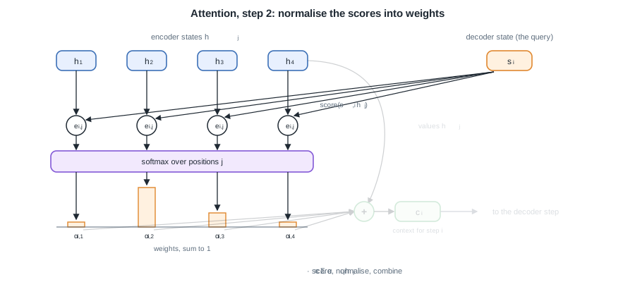
Step 2: the softmax turns the \(T\) scores into weights \(\alpha_{i,j}\) that sum to one, one bar per input position.
9.2.3 Context vector
The context vector for step \(i\) is the weighted average of the encoder states, using the attention weights:
\[\boxed{ c_i = \sum_{j=1}^{T} \alpha_{i,j}\, h_j }\]This \(c_i\) is recomputed at every decoder step, so the model reads a different mixture of the input for each output token. The decoder then combines \(c_i\) with its state \(s_i\) to predict the token, and the alignment weights \(\alpha_{i,j}\) can be visualised as a soft matrix that shows which input words each output word attends to.
Remark: because every step averages over all \(h_j\), no single fixed vector has to carry the whole input. The bottleneck of section 9.1 is gone, and long inputs no longer degrade so quickly.
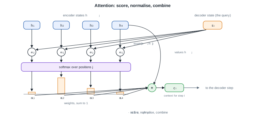
The full mechanism: score, normalise, combine. The context \(c_i\) is the \(\alpha\)-weighted average of the encoder states, rebuilt at every decoder step.
9.3 Score functions
The score function in section 9.2.1 is a design choice. Two forms dominate the early attention literature.
9.3.1 Additive (Bahdanau) score
The additive score, from Bahdanau and co-authors, feeds the two states through a small one-hidden-layer network with learned matrices \(W_1\) and \(W_2\) and a learned vector \(v\):
\[\boxed{ e_{i,j} = v^{\top} \tanh\!\left( W_1 s_i + W_2 h_j \right) }\]It works even when \(s_i\) and \(h_j\) have different dimensions, since \(W_1\) and \(W_2\) project both into a shared space before the \(\tanh\).
9.3.2 Multiplicative (Luong) score
The multiplicative score, from Luong and co-authors, is a plain dot product between the two states:
\[\boxed{ e_{i,j} = s_i^{\top} h_j }\]It has no extra parameters in its simplest form and is far cheaper to compute, since a whole matrix of scores is a single matrix multiplication. A general variant inserts a learned matrix \(W\) as \(s_i^{\top} W h_j\) to handle mismatched dimensions.
9.3.3 Which to use
| Aspect | Additive (Bahdanau) | Multiplicative (Luong) |
|---|---|---|
| Formula | \(v^{\top}\tanh(W_1 s_i + W_2 h_j)\) | \(s_i^{\top} h_j\) |
| Extra parameters | \(W_1\), \(W_2\), \(v\) | none (or one matrix \(W\)) |
| Different dims | handled by projection | needs the \(W\) variant |
| Cost | slower, small network per pair | fast, one matrix product |
| Best when | small models, mixed dimensions | large models, matched dimensions |
Remark: the dot product grows with the dimension of the states, so at large widths its variance gets big and pushes the softmax into flat regions. Scaling the score by \(1/\sqrt{d}\) fixes this, and that scaled dot product is exactly what the Transformer will adopt.
9.4 Query, key, value
Attention has a cleaner reading that drops the encoder-decoder framing. Rename the pieces: the state that does the looking is a query, and each thing that can be looked at contributes a key (used for scoring) and a value (used in the sum).
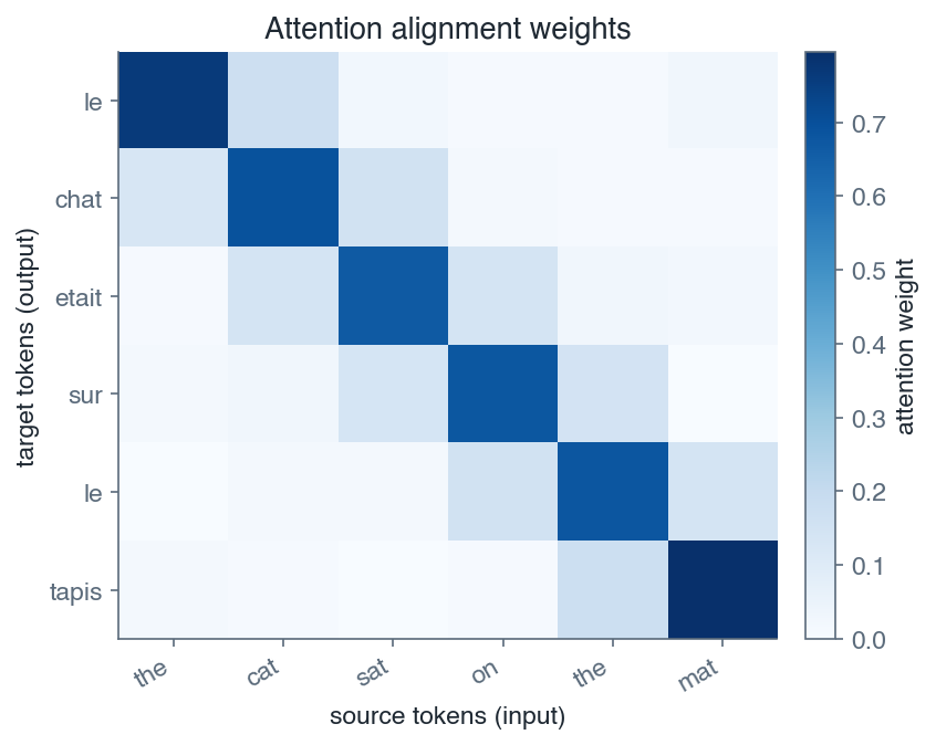
An attention weight matrix: each output token draws mostly from a few input tokens.
\[\boxed{ q = s_i, \quad k_j = h_j, \quad v_j = h_j }\]With this naming the score compares the query against each key, the softmax turns the scores into weights, and the output is the weighted sum of the values:
\[\boxed{ \operatorname{Attention}(q, K, V) = \sum_{j} \operatorname{softmax}_j\!\left(\operatorname{score}(q, k_j)\right) v_j }\]In classic seq2seq attention the key and the value are the same encoder state \(h_j\), but nothing forces that. Separating the three roles is what unlocks the next step.
Remark: in this lesson the query comes from the decoder while the keys and values come from the encoder, so the query attends over a different sequence. When the query, keys, and values all come from the same sequence, each token attends over its own neighbours. That is self-attention, and stacking it is the entire idea behind the Transformer.
Building the query, key, and value from one sequence with learned projections turns attention into a general sequence layer, which is exactly where the next lesson on Transformers begins.
Next: Transformers · Course overview