
7. Recurrent networks
Feedforward and convolutional networks map a fixed-size input to an output in one pass, but many problems come as sequences whose length varies and whose order matters (text, audio, time series). A recurrent neural network (RNN) processes a sequence one step at a time and carries a hidden state forward, so past inputs influence the current output. This module introduces recurrence, the vanilla RNN cell, how it is trained by backpropagation through time, and why long-range gradients tend to vanish or explode.
7.1 Why not an MLP or a CNN?
A sequence is an ordered list of inputs \(x_1, x_2, \dots, x_T\): the words of a review, the samples of an audio clip, the daily values of a time series. Two things make it awkward for the networks we already have. The length \(T\) changes from one example to the next, and the order carries the meaning: "not good, actually great" and "not great, actually good" contain exactly the same words.
Try the tools already on the table:
- An MLP expects one fixed-size vector \(a^{[0]} = x\), so a longer sequence simply does not fit its input layer. Worse, each position gets its own private weights: a pattern learned on the 2nd word teaches nothing about the same pattern on the 9th, the dense-layer problem of lesson 5 all over again, in time instead of space.
- A 1D CNN fixes the sharing: one kernel slides along the sequence, the same weights at every position. But its window is \(k\) steps wide, so two inputs only ever meet if they fall inside the same receptive field. The end of a long sequence cannot see its beginning without stacking many layers, and the reach is still fixed at build time.
What sequences call for is three things at once: accept any length, apply the same weights at every step, and carry a memory of what has been seen so far, however far back.
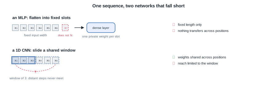
The same six-step sequence, twice. The MLP has fixed slots and private weights per position. The 1D convolution shares its weights, but only relates inputs that fall inside its window.
Whatever meets all three requirements at once will be the subject of this lesson. Before building it, note the shapes sequence tasks come in:
| Setup | Input | Output | Example |
|---|---|---|---|
| Many to one | sequence | single vector | sentiment of a sentence |
| Many to many (aligned) | sequence | sequence, same length | part-of-speech tagging |
| Many to many (seq2seq) | sequence | sequence, other length | machine translation |
| One to many | single vector | sequence | image captioning |
7.2 The vanilla RNN cell
The recurrent network meets all three requirements with one move. It keeps a hidden state (or memory) \(h_t\) that summarizes everything relevant seen up to step \(t\), and it shares one set of parameters across every step, so the same transformation applies whether the sequence has 5 elements or 500. Sharing keeps the parameter count independent of \(T\) and lets a pattern learned at one position generalize to any other.
Remark: weight sharing across time is the sequential analogue of weight sharing across space in a convolutional network. Both encode a prior that the same feature can appear anywhere.
7.2.1 Recurrence
At step \(t\) the cell reads the current input \(x_t\) and the previous hidden state \(h_{t-1}\), then produces a new hidden state through an activation \(g\) (usually \(\tanh\)):
\[\boxed{ h_t = g\left(W_{hh}\, h_{t-1} + W_{xh}\, x_t + b_h\right) }\]The hidden state is initialized to \(h_0 = \mathbf{0}\) (or a learned vector). The per-step output is a linear readout of the hidden state:
\[\boxed{ \hat{y}_t = W_{hy}\, h_t + b_y }\]Here \(W_{hh}\) maps state to state, \(W_{xh}\) maps input to state, and \(W_{hy}\) maps state to output. If the hidden size is \(n_h\) and the input size is \(n_x\), then \(W_{hh}\) is \((n_h \times n_h)\), \(W_{xh}\) is \((n_h \times n_x)\), and \(b_h\) has shape \(n_h\).
Remark: this keeps the explicit-bias convention of the whole Deep Learning course. The bias \(b_h\) is a separate additive term, never folded into the weight matrices the way the Machine Learning course folded the intercept into \(w^T x\) with \(x_0 = 1\).
7.2.2 Shared weights
The crucial point is that \(W_{hh}\), \(W_{xh}\), \(W_{hy}\), \(b_h\), and \(b_y\) do not depend on \(t\). The same five parameters are reused at every step:
\[\boxed{ w = \{W_{hh},\, W_{xh},\, W_{hy},\, b_h,\, b_y\} \quad \text{used at every step } t }\]So an RNN is not a very deep network with distinct layers, it is one small cell applied repeatedly, feeding its own output back as input.
7.3 Unrolling in time
Because the same cell is reused, we can unroll the recurrence into a chain: draw one copy of the cell per time step and connect the hidden state of each copy to the next. The unrolled view is an ordinary feedforward graph (with tied weights), which is exactly what makes gradient computation possible.
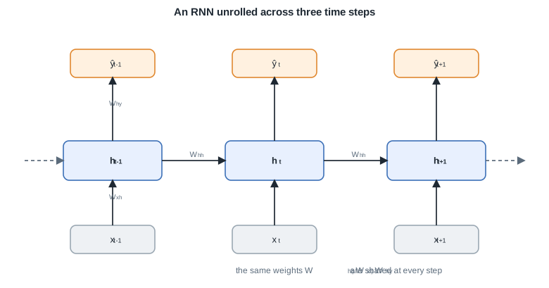
Unrolled in time, a recurrent network reuses the same weights at every step and passes the hidden state forward.
Remark: the horizontal arrows between hidden states are the only path along which information from the past reaches the present. Every one of them multiplies by the same matrix \(W_{hh}\), which is the source of both the model's power and its training difficulty.
7.4 Backpropagation through time
Training minimizes a total cost that sums the per-step loss over the sequence. With per-step loss \(L_t\) comparing \(\hat{y}_t\) to the target \(y_t\), the cost for one sequence is:
\[\boxed{ J = \sum_{t=1}^{T} L_t\left(\hat{y}_t, y_t\right) }\]Backpropagation through time (BPTT) is ordinary backpropagation run on the unrolled graph. Because \(W_{hh}\) is reused at every step, its gradient is the sum of the contributions from all steps:
\[\boxed{ \frac{\partial J}{\partial W_{hh}} = \sum_{t=1}^{T} \frac{\partial L_t}{\partial W_{hh}} }\]For a single step \(t\), the loss depends on \(W_{hh}\) both directly (through \(h_t\)) and indirectly through every earlier hidden state \(h_k\) with \(k \le t\), since each of those was itself produced with \(W_{hh}\). Applying the chain rule through the state chain gives:
\[\boxed{ \frac{\partial L_t}{\partial W_{hh}} = \sum_{k=1}^{t} \frac{\partial L_t}{\partial h_t}\left(\prod_{i=k+1}^{t} \frac{\partial h_i}{\partial h_{i-1}}\right)\frac{\partial h_k}{\partial W_{hh}} }\]Remark: in practice the sum over \(k\) is cut off after a fixed window, which is called truncated BPTT. It bounds memory and compute per update at the cost of ignoring dependencies longer than the window.
7.5 Vanishing and exploding gradients
The inner product \(\prod_{i=k+1}^{t} \frac{\partial h_i}{\partial h_{i-1}}\) is what carries gradient information from step \(t\) back to step \(k\). From the recurrence \(h_i = g(W_{hh} h_{i-1} + W_{xh} x_i + b_h)\), each factor is:
\[\boxed{ \frac{\partial h_i}{\partial h_{i-1}} = \operatorname{diag}\!\left(g'(z_i)\right) W_{hh} }\]where \(z_i = W_{hh} h_{i-1} + W_{xh} x_i + b_h\) is the pre-activation at step \(i\). Composing over the whole gap from \(k\) to \(t\) gives a product of \(t - k\) such matrices:
\[\boxed{ \prod_{i=k+1}^{t} \frac{\partial h_i}{\partial h_{i-1}} = \prod_{i=k+1}^{t} \operatorname{diag}\!\left(g'(z_i)\right) W_{hh} }\]This product of \(t - k\) near-identical factors behaves roughly like a matrix raised to the power \(t - k\). If the relevant magnitude (informally, the largest singular value of \(\operatorname{diag}(g'(z_i)) W_{hh}\)) is below \(1\), the product shrinks geometrically toward zero as the gap grows, so distant gradients vanish. If it is above \(1\), the product blows up and gradients explode.
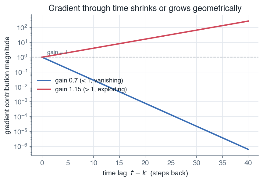
Through many time steps the gradient shrinks or grows geometrically, so long-range dependencies are hard for a plain RNN to learn.
| Regime | Product over time | Effect on training |
|---|---|---|
| Factor magnitude \(< 1\) | decays toward \(0\) | long-range gradients vanish, no long memory learned |
| Factor magnitude \(\approx 1\) | stays bounded | stable, the ideal case |
| Factor magnitude \(> 1\) | grows without bound | gradients explode, updates diverge |
Remark: exploding gradients are usually tamed with gradient clipping (rescale the gradient when its norm exceeds a threshold). Vanishing gradients are harder, because the signal is lost rather than merely large, and no simple rescaling recovers it.
Since a saturating activation such as \(\tanh\) has \(g' \le 1\) everywhere, the diagonal factor tends to pull the product toward vanishing, which makes it hard for a vanilla RNN to learn dependencies more than a few dozen steps apart. This limitation is precisely what motivates gated cells, which add a near-linear path for the state to flow along without repeated squashing.
The next lesson introduces the LSTM and GRU, gated architectures that carry a cell state through additive updates so gradients can travel across long spans without vanishing.
Next: LSTM and GRU · Course overview