
# 6. Embeddings and representation learning Neural networks turn raw inputs into useful features by learning them rather than hand-crafting them. For discrete symbols (words, product IDs, user IDs, categories) the natural representation is a learned dense vector called an embedding. This lesson shows why one-hot codes are a poor input, how an embedding matrix maps each symbol to a compact vector, how word2vec learns such vectors from co-occurrence, and why embeddings are the standard input to the sequence models and Transformers that follow. ## 6.1 From one-hot to dense vectors ### 6.1.1 The one-hot representation Suppose the vocabulary has $V$ distinct symbols. The classic way to feed symbol $i$ to a network is the one-hot vector $x_{\text{onehot}} \in \{0, 1\}^V$, which is all zeros except for a single $1$ at position $i$. It carries no structure: every pair of distinct symbols is exactly as far apart as every other pair, so the code holds no notion of similarity. It is also enormous, a modern vocabulary has $V$ in the tens or hundreds of thousands, and it is almost entirely zeros. | property | one-hot | learned embedding | | --- | --- | --- | | dimension | $V$ (tens of thousands) | $d$ (tens to hundreds) | | sparsity | one nonzero entry | dense, all entries used | | similarity | all pairs equidistant | close vectors mean related symbols | | parameters | none, fixed | learned from data | | downstream size | huge weight matrices | compact, reusable features | *Remark:* feeding a one-hot vector into a linear layer $W x_{\text{onehot}}$ simply selects one column of $W$. The embedding lookup below makes that selection explicit and cheap. ### 6.1.2 The embedding lookup An embedding matrix $E \in \mathbb{R}^{V \times d}$ stores one $d$-dimensional row per symbol. The embedding of a one-hot input is the matrix-vector product $$\boxed{\; e = E^{T} x_{\text{onehot}} \in \mathbb{R}^{d} \;}$$ Because $x_{\text{onehot}}$ has a single $1$ at position $i$, this product just returns row $i$ of $E$, so in practice it is implemented as a table lookup $e = E_{i,:}$ and never as a real multiplication. The vector $e$ is short (dimension $d \ll V$) and dense. *Remark:* the rows of $E$ are ordinary parameters. They start random and are updated by backpropagation together with the rest of the network, so the geometry of the space is shaped by whatever task the network is trained on. ## 6.2 Learning word embeddings with word2vec Embeddings can be learned end to end inside any task, but they can also be learned on their own from unlabelled text. The word2vec skip-gram model does exactly this: it learns a vector per word by predicting the surrounding context words from a centre word. ### 6.2.1 Skip-gram objective Each word $w$ has an input vector $v_w$ (its row in the embedding matrix). Given a centre word $w_I$, the model scores each candidate output word $w_O$ by a dot product and normalizes over the whole vocabulary with a softmax: $$\boxed{\; p(w_O \mid w_I) = \frac{\exp\!\left(v_{w_O}^{T} v_{w_I}\right)}{\sum_{w=1}^{V} \exp\!\left(v_{w}^{T} v_{w_I}\right)} \;}$$ Training maximizes this probability for the (centre, context) pairs that actually co-occur in a sliding window over the text. Words that appear in similar contexts are pushed to have large dot products, so their vectors end up close together. ### 6.2.2 Negative sampling The denominator sums over all $V$ words, which is far too expensive to compute for every training pair. Negative sampling replaces the full softmax with a cheap binary problem: for each real (centre, context) pair, draw a few random words as negatives and train the model to tell the true context word from the fakes. This turns one $V$-way normalization into a handful of logistic updates per step and is what makes word2vec fast enough to train on billions of words. 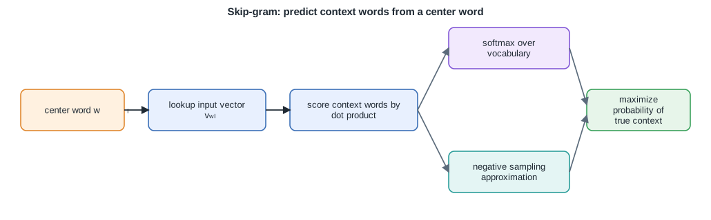 *The skip-gram model learns embeddings by predicting a word context from a center word.* *Remark:* the learned space has a striking linear structure. Directions in it encode consistent relations, so analogies show up as vector arithmetic, the classic example being that the vector for "king" minus "man" plus "woman" lands near "queen". ## 6.3 Measuring similarity Once symbols are dense vectors, "how related are two symbols" becomes a geometric question. The standard answer is cosine similarity, the cosine of the angle between two vectors $u$ and $v$: $$\boxed{\; \cos(u, v) = \frac{u^{T} v}{\lVert u \rVert \, \lVert v \rVert} \;}$$ It lies in $[-1, 1]$: a value near $1$ means the vectors point the same way (very similar), near $0$ means unrelated, and near $-1$ means opposite. Cosine ignores vector length and looks only at direction, which is usually what we want, since a word's meaning should not depend on how often it appears. 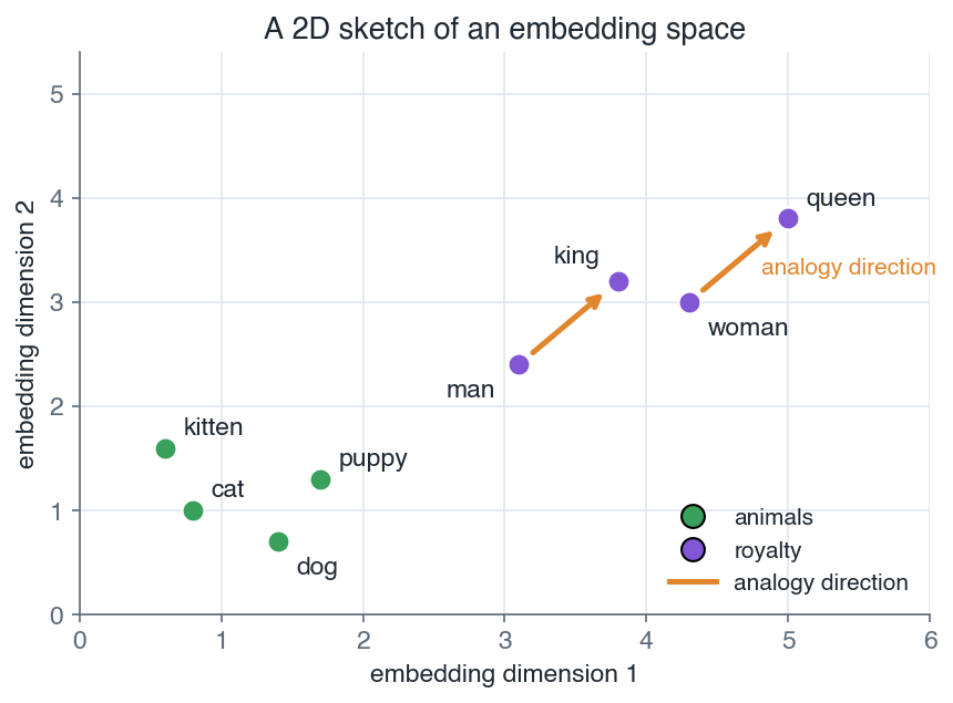 *Learned embeddings place related words near each other, and consistent directions in the space capture analogies.* *Remark:* nearest-neighbour search under cosine similarity is how embeddings power retrieval and recommendation. Find the stored vectors whose direction is closest to a query vector and you have the most relevant items. ## 6.4 Embeddings beyond words Nothing in the construction is specific to language. Any set of discrete symbols can be embedded by giving it a matrix $E$ and learning its rows. | domain | symbol | what the embedding captures | | --- | --- | --- | | language | word or token | meaning and usage | | recommendation | item ID | products bought or viewed together | | recommendation | user ID | a user's taste profile | | tabular data | category level | behaviour of that category | In a recommender, a predicted affinity between a user and an item is read off as the dot product of their embeddings, the same operation that scored words above: $$\boxed{\; \text{score}(\text{user}, \text{item}) = v_{\text{user}}^{T} \, v_{\text{item}} \;}$$ In tabular models, replacing a high-cardinality categorical column with a learned embedding often beats one-hot encoding, because the model can place similar categories near each other instead of treating them as unrelated. *Remark:* embeddings are also a form of dimensionality reduction. They compress a $V$-way symbol into $d$ numbers while keeping the information a downstream task needs, which is the essence of representation learning. ## 6.5 Embeddings as the input to sequence models A sequence of symbols becomes a sequence of vectors by looking each one up in $E$. That matrix of embeddings is exactly the input a recurrent network reads step by step (lesson [Recurrent networks](/en/Deep%20Learning/07%20Recurrent%20networks)) and the input a Transformer attends over (lesson [Transformers](/en/Deep%20Learning/10%20Transformers)). In both cases the embedding table is learned jointly with the rest of the model, so the representations are tuned to the end task rather than fixed in advance. 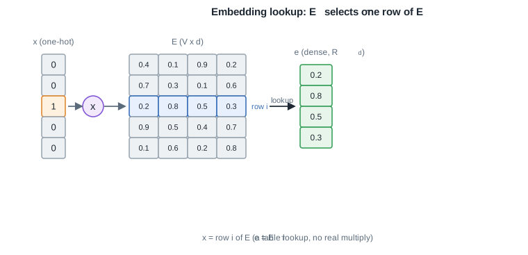 *An embedding lookup selects one row of the matrix E, mapping a sparse one-hot token to a dense learned vector.* *Remark:* pretrained embeddings can be loaded as a starting point and then fine-tuned, so a model does not have to relearn basic semantics from scratch. This transfer of learned representations is one of the reasons deep models generalize so well on limited data. *Dense vectors give us a compact, similarity-aware input. The next lesson feeds such a sequence of vectors, one step at a time, into a recurrent network that carries a hidden state through time.* --- Next: [Recurrent networks](/en/Deep%20Learning/07%20Recurrent%20networks) · [Course overview](/en/Deep%20Learning)