
Blame
|
1 | # 4. Training deep networks |
||||||
| 2 | ||||||||
| 3 | Lesson 3 chose the optimizer. This lesson collects the three tools that make that optimization behave on a deep stack: start the weights at the right scale (initialization), keep the activations well-scaled while they move (normalization), and stop the network from memorizing the training set (regularization). Each deserves a chapter of its own. Here we keep what matters most in practice. |
|||||||
| 4 | ||||||||
| 5 | ## 4.1 Initialization |
|||||||
| 6 | ||||||||
| 7 | **Break the symmetry.** Setting $W^{[l]} = 0$, or any value that makes every unit of a layer identical, breaks learning: two units with the same weights and the same input compute the same activation, receive the same gradient, and stay identical forever. The layer behaves like a single unit no matter how wide it is. Weights therefore start random. Biases can start at zero: the random weights already differ, and a zero bias keeps each unit in the responsive region of its activation. |
|||||||
| 8 | ||||||||
| 9 | **Pick the right scale.** For a unit $z = \sum_{j=1}^{n_{\text{in}}} W_j a_j$ with independent zero-mean weights and inputs, the variance is a sum of $n_{\text{in}}$ terms: |
|||||||
| 10 | ||||||||
| 11 | $$\boxed{ \operatorname{Var}(z) = n_{\text{in}} \cdot \operatorname{Var}(W) \cdot \operatorname{Var}(a) }$$ |
|||||||
| 12 | ||||||||
| 13 | If $n_{\text{in}} \operatorname{Var}(W)$ drifts below $1$ the signal shrinks layer after layer, and lesson 2 proved where that ends: a vanished gradient. Above $1$ it explodes instead. The fix is to hold $n_{\text{in}} \operatorname{Var}(W) \approx 1$, which pins the weight variance to the layer's size: |
|||||||
| 14 | ||||||||
| 15 | $$\boxed{ \text{Xavier: } \operatorname{Var}(W^{[l]}) = \frac{2}{n_{\text{in}} + n_{\text{out}}}, \qquad \text{He: } \operatorname{Var}(W^{[l]}) = \frac{2}{n_{\text{in}}} }$$ |
|||||||
| 16 | ||||||||
| 17 | Xavier (which balances the forward and backward passes) suits $\tanh$ and the sigmoid. He doubles the variance because ReLU zeroes half of its inputs on average, so it is the right target for the ReLU family. |
|||||||
| 18 | ||||||||
| 19 | 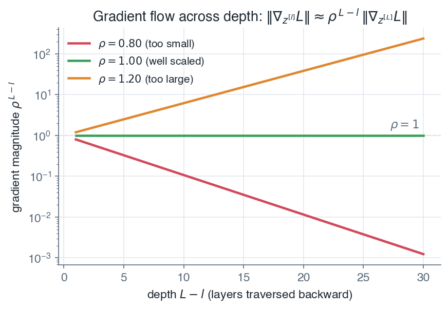 |
|||||||
| 20 | ||||||||
| 21 | *Gradient magnitude across depth: poorly scaled weights make it vanish or explode, while variance-preserving initialization keeps it near one.* |
|||||||
| 22 | ||||||||
| 23 | **Clip what still explodes.** Initialization sets the scale once, at step zero. If gradients still blow up during training (frequent in recurrent networks, lesson 7), rescale the gradient so its norm never exceeds a threshold $\tau$, keeping its direction: |
|||||||
| 24 | ||||||||
| 25 | $$\boxed{ g \leftarrow g \cdot \min\!\left(1, \frac{\tau}{\lVert g \rVert}\right) }$$ |
|||||||
| 26 | ||||||||
| 27 | ## 4.2 Normalization |
|||||||
| 28 | ||||||||
| 29 | Initialization only positions the network at step zero: as training moves the weights, the distribution of every layer's input drifts, and later layers keep chasing a moving target. A normalization layer fixes the statistics on the fly: standardize, then let the network learn its scale back. For a feature $x$ over a mini-batch of size $m$, batch normalization computes |
|||||||
| 30 | ||||||||
| 31 | $$\boxed{ \mu_\mathcal{B} = \frac{1}{m}\sum_{i=1}^{m} x^{(i)}, \qquad \sigma_\mathcal{B}^2 = \frac{1}{m}\sum_{i=1}^{m}\left(x^{(i)} - \mu_\mathcal{B}\right)^2 }$$ |
|||||||
| 32 | ||||||||
| 33 | $$\boxed{ \hat{x}^{(i)} = \frac{x^{(i)} - \mu_\mathcal{B}}{\sqrt{\sigma_\mathcal{B}^2 + \epsilon}}, \qquad y^{(i)} = \gamma\, \hat{x}^{(i)} + \beta }$$ |
|||||||
| 34 | ||||||||
| 35 | The scale $\gamma$ and shift $\beta$ are learned like any weight, so normalization removes no capacity: the network can even learn to undo it. The payoff is a smoother loss surface, higher usable learning rates, and less sensitivity to initialization. Two practical consequences: at inference, where there is no batch, BatchNorm switches to running averages of $\mu$ and $\sigma^2$ accumulated during training (forgetting that switch is the classic BatchNorm bug), and the shift $\beta$ makes the layer bias $b^{[l]}$ redundant. |
|||||||
| 36 | ||||||||
| 37 | Layer normalization keeps the same standardize-scale-shift recipe but averages over the features of a single example instead of over the batch. Its statistics no longer depend on the batch, so it behaves identically in training and inference and handles variable-length sequences, which makes it the choice for recurrent networks and Transformers (lesson 10). |
|||||||
| 38 | ||||||||
| 39 | | Aspect | Batch normalization | Layer normalization | |
|||||||
| 40 | | --- | --- | --- | |
|||||||
| 41 | | Normalization axis | across the batch, per feature | across the features, per example | |
|||||||
| 42 | | Train vs inference | batch statistics vs running statistics | identical in both | |
|||||||
| 43 | | Typical use | CNNs and feedforward vision models | RNNs and Transformers | |
|||||||
| 44 | ||||||||
| 45 | 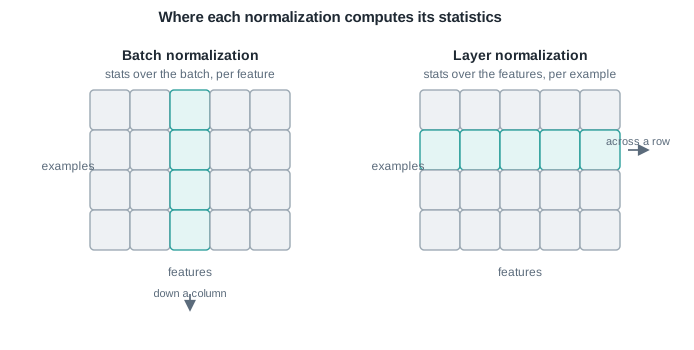 |
|||||||
| 46 | ||||||||
| 47 | *Batch normalization computes statistics down a feature column across the batch, layer normalization across the features of a single example.* |
|||||||
| 48 | ||||||||
| 49 | ## 4.3 Regularization and dropout |
|||||||
| 50 | ||||||||
| 51 | A deep network usually has more parameters than training examples, so it can memorize the training set, noise included. Regularization trades a little training accuracy for generalization, the bias-variance story of [General concepts](/en/Machine%20Learning/02%20General%20concepts). |
|||||||
| 52 | ||||||||
| 53 | **Weight decay ($L_2$).** Add a penalty on the squared weights to the cost, with strength $\lambda$: |
|||||||
| 54 | ||||||||
| 55 | $$\boxed{ J_{\text{reg}} = J + \frac{\lambda}{2}\sum_{l=1}^{L}\lVert W^{[l]} \rVert_F^2 \quad\Longrightarrow\quad W^{[l]} \leftarrow (1 - \alpha\lambda)\, W^{[l]} - \alpha\,\frac{\partial J}{\partial W^{[l]}} }$$ |
|||||||
| 56 | ||||||||
| 57 | The factor $(1 - \alpha\lambda)$ shrinks every weight at every step, hence the name. Its $L_1$ cousin penalizes absolute values instead and drives many weights to exactly zero. Biases are left out of the penalty. |
|||||||
| 58 | ||||||||
| 59 | **Dropout.** On each training pass, keep every unit with probability $p$ and zero it otherwise, then divide by $p$ so the expected signal is unchanged: |
|||||||
| 60 | ||||||||
| 61 | $$\boxed{ \tilde{a}^{[l]} = \frac{m \odot a^{[l]}}{p}, \qquad m_i \sim \text{Bernoulli}(p) }$$ |
|||||||
| 62 | ||||||||
| 63 | No unit can rely on its neighbours, so the representation spreads out. Each step trains one of $2^k$ thinned subnetworks that share their weights, and inference, with dropout off, approximates their average prediction for free (that is what the $1/p$ buys). Typical keep probabilities: around $0.8$ at the input, $0.5$ in hidden layers. |
|||||||
| 64 | ||||||||
| 65 | 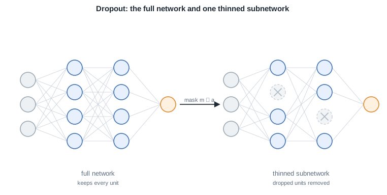 |
|||||||
| 66 | ||||||||
| 67 | *Dropout trains a different thinned subnetwork on each step by randomly removing units, and averages them at inference.* |
|||||||
| 68 | ||||||||
| 69 | *Initialized at the right scale, normalized in flight, and regularized against memorizing, the network is ready for architecture. The next lesson builds the convolutional network, whose weight sharing is itself a form of regularization.* |
|||||||
| 70 | ||||||||
| 71 | --- |
|||||||
| 72 | Next: [Convolutional networks](/en/Deep%20Learning/05%20Convolutional%20networks) · [Course overview](/en/Deep%20Learning) |
|||||||