
# 3. Optimization Backpropagation returns the gradient of the cost with respect to every parameter. An optimizer is the rule that turns those gradients into updates. This module covers the gradient-descent variants and the adaptive optimizers (momentum, RMSProp, Adam) that make deep networks trainable, plus the learning-rate schedules that shape the run. ## 3.1 Gradient descent Let $w$ collect all parameters (every $W^{[l]}$ and $b^{[l]}$) and let $J(w)$ be the cost, the average of the per-example loss $L$. Write $g = \nabla_w J(w)$ for the gradient of the cost with respect to the parameters, as returned by backpropagation. The base update moves $w$ downhill: $$\boxed{ w \leftarrow w - \alpha\, g }$$ with learning rate $\alpha > 0$. This is the LMS update from the Machine Learning course, written for the full parameter vector instead of one coordinate. *Remark:* bias is explicit here. The gradient $g$ has one block per $W^{[l]}$ and one per $b^{[l]}$, and the update applies to each block with the same $\alpha$. ### 3.1.1 Batch, mini-batch, stochastic The variants differ only in how many examples enter the gradient $g$ at each step. | variant | examples per step | update noise | per step | use when | | --- | --- | --- | --- | --- | | Batch GD | all $m$ | none | $O(m)$ passes | $m$ small, exact gradient wanted | | Mini-batch GD | a batch of $B$ | moderate | $O(B)$ | the default for deep nets | | Stochastic GD (SGD) | one example | high | $O(1)$ | streaming, very large $m$ | *Remark:* one pass over the whole dataset is an epoch. Mini-batch is the standard choice: batches of $32$ to $512$ fit the accelerator, exploit vectorized matrix products, and the residual noise in $g$ helps escape shallow local minima. In deep learning "SGD" is used loosely to mean mini-batch gradient descent. ## 3.2 Momentum Plain SGD zig-zags across narrow valleys because the gradient points across the valley more than along it. Momentum accumulates an exponentially weighted average of past gradients in a velocity vector $v$, then steps in that averaged direction: $$\boxed{ v \leftarrow \beta\, v + g, \qquad w \leftarrow w - \alpha\, v }$$ with momentum coefficient $\beta \in [0, 1)$, typically $\beta = 0.9$. Components of $g$ that keep the same sign reinforce each other, so $v$ grows and the step accelerates along consistent directions. Components that flip sign cancel in the average, so oscillations across the valley are damped.  *The curves are level lines of the loss, the dot is the minimum. The gradient is perpendicular to the level line it sits on, so in a ravine it points mostly across the valley, and plain gradient descent bounces. Momentum keeps a memory of the previous steps, the bounces cancel and the valley direction accumulates.* ### 3.2.1 Nesterov momentum Nesterov accelerated gradient evaluates the gradient at a look-ahead point, after the momentum step has been provisionally applied, rather than at the current $w$. This anticipatory correction reacts sooner when the slope changes: $$\boxed{ v \leftarrow \beta\, v + \nabla_w J(w - \alpha \beta\, v), \qquad w \leftarrow w - \alpha\, v }$$ *Remark:* think of $\beta \approx 0.9$ as averaging over roughly the last $\tfrac{1}{1 - \beta} = 10$ gradients. Nesterov usually converges slightly faster than plain momentum for the same $\alpha$ and $\beta$. ## 3.3 RMSProp Different parameters can need very different step sizes, and one global $\alpha$ cannot serve them all. RMSProp keeps a per-coordinate running average $s$ of squared gradients, then divides the step by $\sqrt{s}$, so coordinates with large recent gradients take smaller steps and quiet coordinates take larger ones: $$\boxed{ s \leftarrow \rho\, s + (1 - \rho)\, g^2, \qquad w \leftarrow w - \alpha\, \frac{g}{\sqrt{s} + \epsilon} }$$ with decay $\rho \approx 0.9$ and a small $\epsilon \approx 10^{-8}$ for numerical safety. Here $g^2 = g \odot g$ is the Hadamard (elementwise) square and the division is elementwise, so each coordinate is normalized by its own recent gradient scale. *Remark:* $s$ estimates the uncentered second moment of each coordinate of $g$, so $\sqrt{s}$ is roughly its recent root-mean-square magnitude. RMSProp suits non-stationary objectives, which is exactly what a moving mini-batch gradient is. ## 3.4 Adam Adam (adaptive moment estimation) combines momentum and RMSProp: it keeps a first-moment estimate $m$ (the mean of the gradient) and a second-moment estimate $v$ (the mean of the squared gradient). $$\boxed{ m \leftarrow \beta_1\, m + (1 - \beta_1)\, g, \qquad v \leftarrow \beta_2\, v + (1 - \beta_2)\, g^2 }$$ Both $m$ and $v$ start at zero, so early in training they are biased toward zero. Dividing by $1 - \beta_1^t$ and $1 - \beta_2^t$ at step $t$ removes that bias: $$\boxed{ \hat m = \frac{m}{1 - \beta_1^{\,t}}, \qquad \hat v = \frac{v}{1 - \beta_2^{\,t}} }$$ The update then steps in the momentum direction, rescaled per coordinate by the second moment: $$\boxed{ w \leftarrow w - \alpha\, \frac{\hat m}{\sqrt{\hat v} + \epsilon} }$$ Common defaults are $\beta_1 = 0.9$, $\beta_2 = 0.999$, and $\epsilon = 10^{-8}$. As before the square, square root, and division are elementwise. *Remark:* the bias correction matters most in the first few dozen steps, when $t$ is small and $\beta_2^t$ is still close to $1$. Without it, $\hat v$ would be far too small and the early steps far too large. AdamW, a common variant, decouples weight decay from this update. 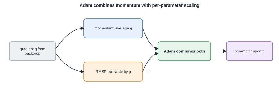 *Adam combines the momentum of averaged gradients with the per-parameter scaling of RMSProp.* ## 3.5 Learning-rate schedules The learning rate $\alpha$ is the single most important hyperparameter, and holding it fixed is rarely optimal. A large $\alpha$ speeds early progress but prevents settling into a minimum, so schedules typically decrease $\alpha$ over training. Here $\alpha_0$ is the initial rate and $t$ indexes the step or epoch. ### 3.5.1 Step decay Multiply $\alpha$ by a factor $\gamma \in (0, 1)$ every $s$ epochs, so it drops in discrete stages: $$\boxed{ \alpha_t = \alpha_0\, \gamma^{\lfloor t / s \rfloor} }$$ ### 3.5.2 Cosine decay Anneal $\alpha$ smoothly from $\alpha_0$ toward a floor of zero along a half cosine over $T$ total steps: $$\boxed{ \alpha_t = \tfrac{1}{2}\,\alpha_0\left(1 + \cos\frac{\pi t}{T}\right) }$$ ### 3.5.3 Warmup Warmup ramps $\alpha$ up linearly from a small value over the first few hundred to few thousand steps, then hands off to a decay schedule. It prevents the large, poorly conditioned updates a cold start with a big $\alpha$ would produce, and it is standard for deep networks such as transformers. | schedule | shape | main use | | --- | --- | --- | | Step decay | staircase drops | classic vision training | | Cosine | smooth anneal to zero | modern default, often with warmup | | Warmup | linear ramp up, then decay | stabilize early steps, large models | 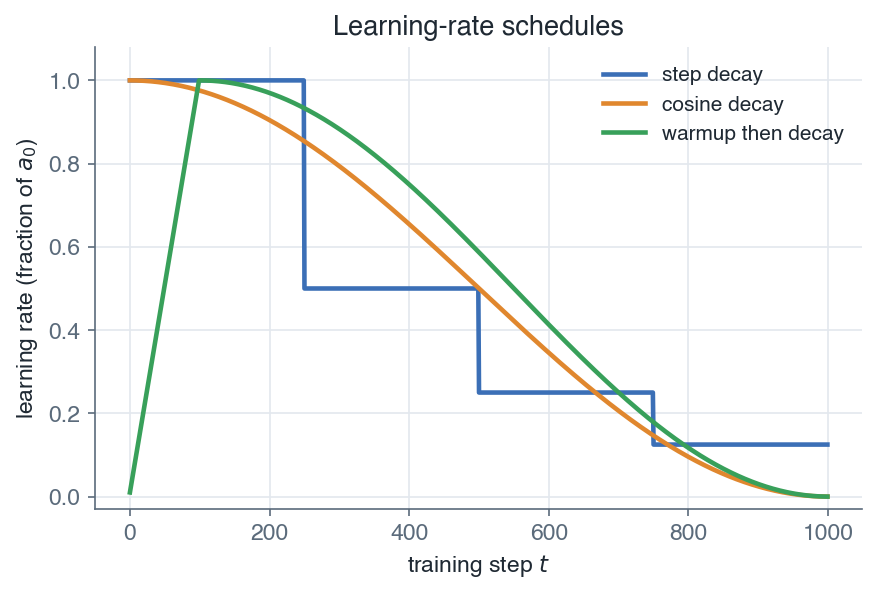 *Common learning-rate schedules: step decay, cosine decay, and a warmup followed by decay.* *Remark:* warmup and a decay are usually composed, warmup for the first phase and cosine or step decay afterward. ## 3.6 Choosing an optimizer | optimizer | what it adds | tracks | typical use | | --- | --- | --- | --- | | SGD | nothing, base rule | none | strong baseline, best final accuracy with tuning | | Momentum | velocity, damps oscillation | first moment $v$ | vision models, with a schedule | | RMSProp | per-coordinate scaling | second moment $s$ | RNNs, non-stationary objectives | | Adam | momentum plus scaling, bias-corrected | first and second moments | the default first choice for most nets | *Remark:* Adam is the safe default and converges fast with little tuning. Well-tuned SGD with momentum and a schedule often reaches slightly better final test accuracy on large vision models, which is why both remain in wide use. 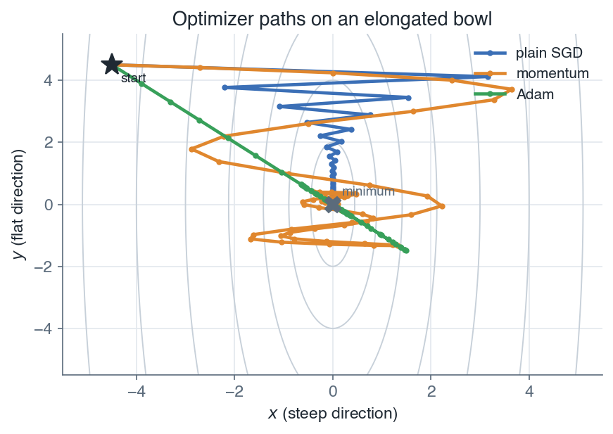 *On an elongated loss surface, momentum and Adam reach the minimum far faster than plain gradient descent.* ## 3.7 Good practices Two of the habits that make training behave, careful initialization and dropout, live in the next lesson ([Training deep networks](/en/Deep%20Learning/04%20Training%20deep%20networks)). Two more belong right here. **Center and normalize the inputs.** Standardize each feature (subtract its mean, divide by its standard deviation), so no feature dominates the first dot products and the first layer's gradients start well scaled. **Sanity-check before training long.** A freshly initialized $K$-class classifier should start near the loss $\ln K$ (about $2.3$ for $K = 10$). A tiny training set should be easy to overfit: if the network cannot, the code is broken. Watch the training and validation curves. And since backpropagation is error-prone, check its analytic gradient against a numerical finite-difference estimate: $$\boxed{ \frac{\partial L}{\partial w} \approx \frac{L(w + \varepsilon) - L(w - \varepsilon)}{2\varepsilon} }$$ *Every optimizer here scales the raw gradient, so its behaviour depends on how large those gradients are to begin with. The next part studies how the initial weights and the network depth set that scale, and how poor choices make gradients vanish or explode.* --- Next: [Training deep networks](/en/Deep%20Learning/04%20Training%20deep%20networks) · [Course overview](/en/Deep%20Learning)