
# 2. Activation functions Each layer computes a pre-activation $z^{[l]} = W^{[l]} a^{[l-1]} + b^{[l]}$ and then an activation $a^{[l]} = g^{[l]}(z^{[l]})$. The choice of the nonlinearity $g^{[l]}$ is what makes depth worthwhile. This lesson explains why a nonlinear $g$ is required, surveys the sigmoid, tanh, and ReLU families, introduces the softmax used at the output, and gives practical guidance on which activation to pick. ## 2.1 Why nonlinearity is required Suppose every activation were the identity, $g^{[l]}(z) = z$. Then each layer is just $a^{[l]} = W^{[l]} a^{[l-1]} + b^{[l]}$, and composing two of them gives $W^{[2]}(W^{[1]} x + b^{[1]}) + b^{[2]} = (W^{[2]} W^{[1]}) x + (W^{[2]} b^{[1]} + b^{[2]})$. That is again of the form $W x + b$. By induction the whole $L$-layer network reduces to a single affine map: $$\boxed{ g^{[l]} = \text{identity} \;\Rightarrow\; \hat{y} = W' x + b' }$$ with $W' = W^{[L]} \cdots W^{[1]}$ and $b'$ the accumulated bias. No matter how many linear layers are stacked, the model can only fit a linear function, so the extra depth buys nothing. A nonlinear $g$ between layers is exactly what breaks this collapse and lets the network represent curved decision boundaries and nonlinear regressions. *Remark:* the bias is kept explicit here as $b^{[l]}$, unlike the Machine Learning course where the intercept was folded into $w^T x$ via the augmented input $x_0 = 1$. In this Deep Learning course each layer has its own weight matrix $W^{[l]}$ and its own bias vector $b^{[l]}$. ## 2.2 Sigmoid and tanh 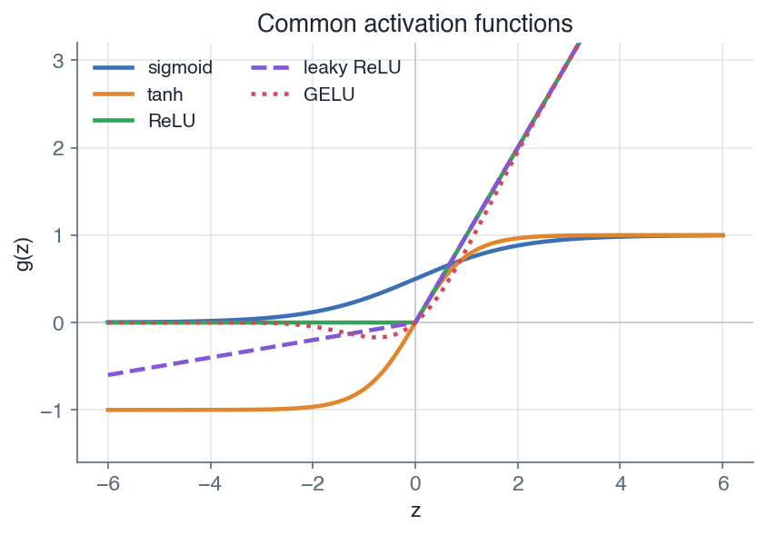 *Common activation functions: the bounded sigmoid and tanh saturate in their tails, while ReLU and its variants stay linear for positive inputs.* ### 2.2.1 Sigmoid The sigmoid squashes any real pre-activation into the open interval $(0, 1)$: $$\boxed{ \sigma(z) = \frac{1}{1 + e^{-z}} \in (0, 1) }$$ Its derivative has the convenient closed form below, which reuses the forward value $\sigma(z)$ already computed: $$\boxed{ \sigma'(z) = \sigma(z)\left(1 - \sigma(z)\right) }$$ ### 2.2.2 Tanh The hyperbolic tangent is a rescaled sigmoid centred at zero, with output in $(-1, 1)$. Its derivative is likewise expressible from the forward value: $$\boxed{ \tanh'(z) = 1 - \tanh(z)^2 }$$ *Remark:* $\tanh$ is zero-centred while $\sigma$ is not, so $\tanh$ often trains a little better as a hidden activation. The two are related by $\tanh(z) = 2\sigma(2z) - 1$. ### 2.2.3 Saturation Both curves flatten in their tails. For large $|z|$ the output is close to a constant ($0$ or $1$ for $\sigma$, $\pm 1$ for $\tanh$), so the derivative is close to zero: $\sigma'(z) \to 0$ and $\tanh'(z) \to 0$. A unit sitting in that flat region is said to saturate, and it passes almost no gradient backward. When many such factors multiply through a deep stack the gradient shrinks toward zero: the vanishing gradient, made precise in the next section. 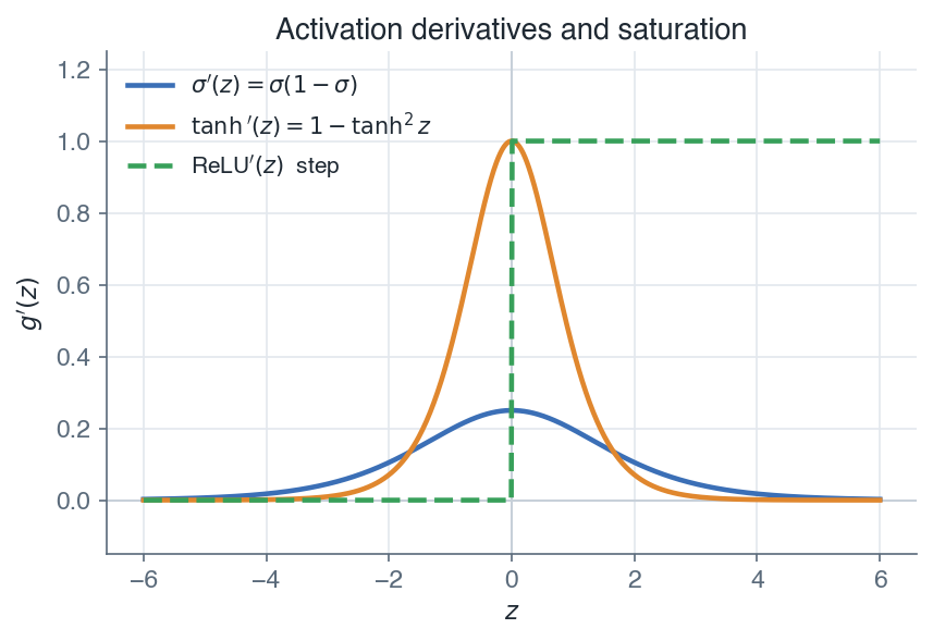 *Activation derivatives: sigmoid and tanh gradients vanish in the tails, whereas the ReLU gradient is 1 wherever the unit is active.* ## 2.3 The vanishing gradient Saturation is not a cosmetic flaw, it decides whether a deep stack can train at all. Backpropagation multiplies the error by the local slope $g'(z^{[l]})$ at every layer it crosses, so the gradient reaching layer 1 contains one such factor per layer. With sigmoid activations those factors are small by construction: section 2.2.1 gave $\sigma'(z) = \sigma(z)(1 - \sigma(z))$, and that product never exceeds $$\boxed{ \sigma'(z) = \sigma(z)\left(1 - \sigma(z)\right) \le \tfrac{1}{4} }$$ The result is the vanishing gradient: the layers near the output learn, the layers near the input receive almost nothing and barely move. Deep sigmoid networks stall, and the fix is not a better optimizer, it is a better activation, the ReLU of the next section. <details class="proof"> <summary>Proof: the gradient shrinks geometrically with depth</summary> **Step 1: the sigmoid's slope never exceeds $1/4$.** Write $s = \sigma(z) \in (0, 1)$. The product $s(1 - s)$ is a downward parabola in $s$, largest at $s = \tfrac{1}{2}$ where it equals $\tfrac{1}{4}$. So the bound holds, with equality only at $z = 0$, and saturation makes it far worse: a unit sitting at $\sigma(2) \approx 0.88$ already has slope $0.88 \cdot 0.12 \approx 0.10$. **Step 2: backpropagation multiplies those slopes.** Take the simplest deep network, a chain of $L$ layers with one unit each, so every quantity is a scalar. Each layer crossed contributes the factor $\partial z^{[l]} / \partial z^{[l-1]} = w^{[l]}\, \sigma'(z^{[l-1]})$: $$\frac{\partial L}{\partial z^{[1]}} = \frac{\partial L}{\partial z^{[L]}} \prod_{l=2}^{L} w^{[l]}\, \sigma'(z^{[l-1]})$$ With weights of typical size $|w^{[l]}| \le 1$, every factor is at most $\tfrac{1}{4}$ in absolute value, so $$\boxed{ \left|\frac{\partial L}{\partial z^{[1]}}\right| \le \left(\tfrac{1}{4}\right)^{L-1} \left|\frac{\partial L}{\partial z^{[L]}}\right| }$$ Ten layers already shrink the gradient by about $10^{-6}$. $\blacksquare$ </details> Weights much larger than $1$ only trade the problem for its mirror image, the exploding gradient. [Training deep networks](/en/Deep%20Learning/04%20Training%20deep%20networks) picks the weight scale so this product stays near $1$. ## 2.4 The ReLU family The rectified linear unit keeps the positive part of its input and zeroes the rest: $$\boxed{ \text{ReLU}(z) = \max(0, z) }$$ Its derivative is $1$ for $z > 0$ and $0$ for $z < 0$ (undefined at $z = 0$, taken to be $0$ or $1$ by convention). ReLU does not saturate on the positive side, so it keeps a healthy gradient flowing there, which is a large part of why it became the default hidden activation. The cost is the dead-unit problem: if a unit's pre-activation is always negative across the data, its gradient is always zero and it stops learning entirely. The variants below trade a little simplicity to soften that failure or to smooth the kink at the origin. | name | formula | derivative | dies / saturates? | | --- | --- | --- | --- | | ReLU | $\max(0, z)$ | $1$ if $z>0$ else $0$ | can die (zero gradient for $z<0$) | | Leaky ReLU | $\max(\alpha z, z)$, $\alpha \approx 0.01$ | $1$ if $z>0$ else $\alpha$ | rarely dies (small negative slope) | | PReLU | $\max(\alpha z, z)$, $\alpha$ learned | $1$ if $z>0$ else $\alpha$ | rarely dies ($\alpha$ trained per channel) | | ELU | $z$ if $z>0$ else $\alpha(e^z - 1)$ | $1$ if $z>0$ else $\alpha e^z$ | saturates gently for $z\to-\infty$ | | GELU | $z\,\Phi(z)$, $\Phi$ the normal CDF | smooth, near $1$ for large $z$ | smooth, no hard death | *Remark:* leaky ReLU and PReLU add a small slope $\alpha$ on the negative side so a unit is never fully switched off. GELU weights the input by the probability $\Phi(z)$ that a standard normal is below $z$, giving a smooth curve that behaves like ReLU for large $|z|$. It is the standard choice inside Transformers. ## 2.5 Softmax for multiclass outputs For a classification with $K$ classes the final layer outputs a vector $z \in \mathbb{R}^K$ of scores, and the softmax turns it into a probability distribution over the classes: $$\boxed{ \text{softmax}(z)_k = \frac{e^{z_k}}{\sum_{j=1}^{K} e^{z_j}} }$$ Each component lies in $(0, 1)$ and the components sum to $1$, so $\text{softmax}(z)_k$ reads as the predicted probability of class $k$. The largest score becomes the most likely class. *Remark:* softmax belongs at the output layer, not in a hidden layer. It couples every unit through the shared denominator (a normalization across the whole vector), which is exactly what a probability output needs but is not a useful per-unit hidden nonlinearity. For a single output ($K = 1$ vs its complement) softmax reduces to the sigmoid. The pairing of softmax with its loss was settled in section 6.3 of [Multilayer neural networks](/en/Machine%20Learning/06%20Multilayer%20neural%20networks). ## 2.6 Choosing an activation A useful default: use ReLU or GELU in the hidden layers, and choose the output activation from the task. The diagram and table below summarize the decision. 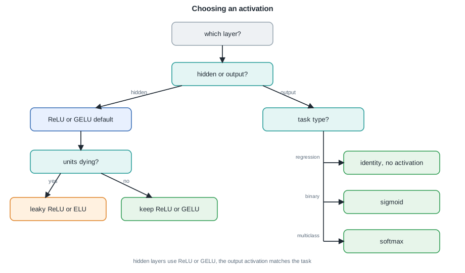 *Choosing an activation: ReLU or GELU for hidden layers, and an output activation matched to the task.* | layer / task | recommended activation | reason | | --- | --- | --- | | hidden (default) | ReLU or GELU | no positive-side saturation, cheap, trains fast | | hidden (dead units) | leaky ReLU or ELU | keeps a nonzero gradient for $z < 0$ | | output, regression | identity (none) | prediction is an unbounded real value | | output, binary | sigmoid | maps score to a probability in $(0, 1)$ | | output, multiclass | softmax | maps scores to a distribution over classes | *Remark:* sigmoid and tanh are now rarely used as hidden activations in deep feed-forward networks precisely because of the saturation in Section 3.2.3. They survive at the output (sigmoid) and inside gated recurrent units, where their bounded range is the point. *With the per-layer nonlinearities fixed, the next lesson turns the gradients into updates: the optimizers that make deep training practical.* --- Next: [Optimization](/en/Deep%20Learning/03%20Optimization) · [Course overview](/en/Deep%20Learning)